Correlation ABI, NPP and EVI

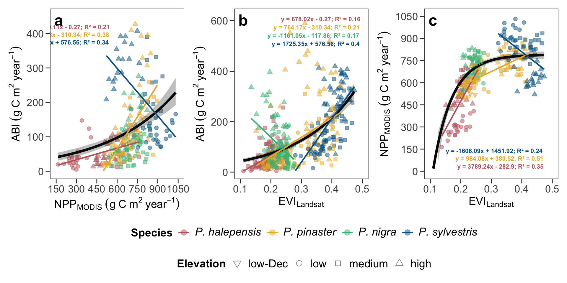
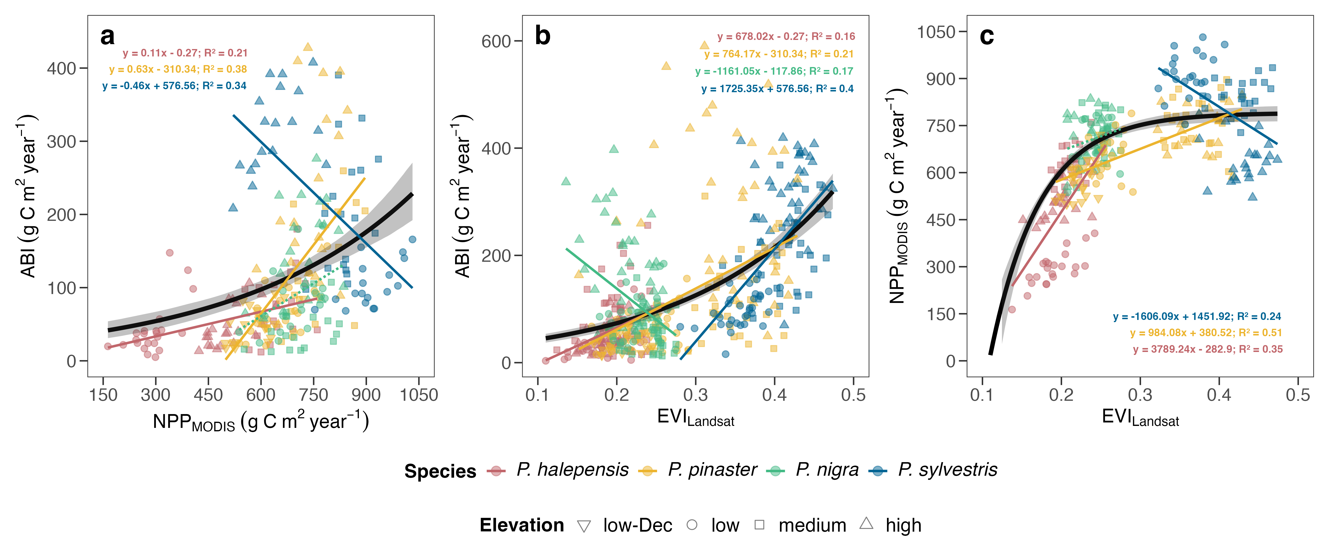
• This figure corresponds to figure 4 in the manuscript.
• An high-resolution version of this figure is available here.

# pkgs 
library(tidyverse)
library(boot)
library(patchwork)
library(here)
library(glue)
library(broom)
source(here::here("scripts/aux.R"))

options(scipen = 999)

# Read data
## A
abi <- read_csv(here::here("data/abi.csv")) |> 
  mutate(se = NA, sd = NA, variable = "abi") |> 
  rename(mean = abi)

## EVI Landsat 
evi_landsat <- read_csv(here::here("data/iv_landsat.csv")) |>
  filter(iv == "evi") |>
  dplyr::select(year, sp_code, elev_code, sp_elev, mean, sd, se) |>
  mutate(variable = "evi_landsat")

npp <- read_csv(here::here("data/npp_modis.csv")) |>
  rename(mean = npp) |>
  mutate(se = NA, sd = NA, variable = "npp") |>
  dplyr::select(year, sp_code, elev_code, sp_elev, mean, sd, se, variable)


df_index <- bind_rows(
  abi, evi_landsat, npp
) |>
  mutate(elev_code = fct_relevel(elev_code, "low-Dec", "low", "medium", "high")) |>
  mutate(sp_code = fct_relevel(sp_code, "halepensis","pinaster", "nigra", "sylvestris")) |> 
  mutate(Specie = paste0("P. ", sp_code)) |>
  mutate(Specie = fct_relevel(Specie, "P. halepensis","P. pinaster", "P. nigra", "P. sylvestris")) |> 
  rename(mean_y = mean, y_variable = variable) 

abi_npp <- df_index |>
  filter(y_variable %in% c("abi", "npp")) |>
  dplyr::select(-se, -sd) |>
  pivot_wider(values_from = mean_y, names_from = y_variable) |>
  filter(!is.na(npp)) |>
  filter(!is.na(abi)) |>
  rowwise() |>
  mutate(ratio = abi / npp)


## ABI vs NPP
# Generate a confidence interval with bootstrap
# Define a function to perform the bootstrapping
boot_func_abi_npp <- function(data, indices) {
  # Take a bootstrap sample
  sample_df <- data[indices, ]
  # Fit the non-linear model
  nls_fit <- nls(abi ~ a * exp(b * npp), data = sample_df, start = list(a = 10, b = 0.002958839))
  # Generate predicted values for a sequence of npp
  npp_seq <- seq(min(data$npp), max(data$npp), length.out = 100)
  pred <- predict(nls_fit, newdata = data.frame(npp = npp_seq))
  return(pred)
}


# Perform bootstrapping with 1000 resamples
boot_res_abi_npp <- boot(data = abi_npp, statistic = boot_func_abi_npp, R = 1000) # R is the number of resamples


# Compute the 95% confidence intervals for each point
ci_lower <- apply(boot_res_abi_npp$t, 2, quantile, probs = 0.025) # Lower 2.5%
ci_upper <- apply(boot_res_abi_npp$t, 2, quantile, probs = 0.975) # Upper 97.5%

# Predicted values from the original fit
npp_seq <- seq(min(abi_npp$npp), max(abi_npp$npp), length.out = 100)
pred_abi_npp <- apply(boot_res_abi_npp$t, 2, mean) # Mean of the bootstrapped predictions

# Create a data frame with predicted values and confidence intervals
pred_df_abi_npp <- data.frame(
  npp = npp_seq,
  abi = pred_abi_npp,
  ci_lower = ci_lower,
  ci_upper = ci_upper
)

labi_npp <- abi_npp |> 
  group_by(sp_code) |> 
  group_modify(~ {
    # Ajusta el modelo
    mod <- lm(abi ~ npp, data = .x)
    # Tidy con coeficientes
    tidy_df <- broom::tidy(mod)
    # Añade R2 a cada fila
    tidy_df$r.squared <- broom::glance(mod)$r.squared
    
    tidy_df
  }) |> 
  mutate(p = case_when(
    p.value < 0.001 ~ "<0.001",
    p.value >= 0.001 ~ as.character(round(p.value, 3))
  )) |> 
  mutate(sig = case_when(
    p.value < 0.001 ~ "sig",
    p.value >= 0.001 ~ "no sig"  
  )) 

y_max_abi <- 450

labi_npp_eq <- labi_npp |> 
  left_join(
    labi_npp |> filter(term == "(Intercept)") |> 
      dplyr::select(sp_code, intercept = estimate)
  ) |> 
  mutate(
    eq_text = if_else(
      sig == "sig", 
      glue("y = {round(estimate, 2)}x {ifelse(intercept < 0, '-', '+')} {round(abs(intercept), 2)}; R² = {round(r.squared, 2)}"),
     NA
    )
  ) |> 
  filter(term != "(Intercept)") |> 
  arrange(desc(sig)) |> # ordenar por eq 
  rowid_to_column("id") |> 
  mutate(offset_y = id * 0.05 * y_max_abi, 
         y_max = y_max_abi - offset_y) |> 
  mutate(Specie = paste0("P. ", sp_code))


abi_npp <- 
  abi_npp |> inner_join(
    labi_npp_eq|> dplyr::select(sp_code, p, sig))


## ABI vs EVI
abi_evi <- df_index |>
  filter(y_variable %in% c("abi", "evi_landsat")) |>
  dplyr::select(-se, -sd) |>
  pivot_wider(values_from = mean_y, names_from = y_variable) |>
  filter(!is.na(evi_landsat)) |>
  filter(!is.na(abi))


# Generate a confidence interval with bootstrap
# Define a function to perform the bootstrapping
boot_func_abi_evi <- function(data, indices) {
  # Take a bootstrap sample
  sample_df <- data[indices, ]
  # Fit the non-linear model
  nls_fit <- nls(abi ~ a * exp(b * evi_landsat), data = sample_df, start = list(a = 15, b = 6.128))
  # Generate predicted values for a sequence of npp
  evi_seq <- seq(min(data$evi_landsat), max(data$evi_landsat), length.out = 100)
  pred <- predict(nls_fit, newdata = data.frame(evi_landsat = evi_seq))
  return(pred)
}

# Perform bootstrapping with 1000 resamples
boot_res_abi_evi <- boot(data = abi_evi, statistic = boot_func_abi_evi, R = 1000) # R is the number of resamples

# Compute the 95% confidence intervals for each point
ci_lower <- apply(boot_res_abi_evi$t, 2, quantile, probs = 0.025) # Lower 2.5%
ci_upper <- apply(boot_res_abi_evi$t, 2, quantile, probs = 0.975) # Upper 97.5%

# Predicted values from the original fit
evi_seq <- seq(min(abi_evi$evi_landsat), max(abi_evi$evi_landsat), length.out = 100)
pred_abi_evi <- apply(boot_res_abi_evi$t, 2, mean) # Mean of the bootstrapped predictions

# Create a data frame with predicted values and confidence intervals
pred_df_abi_evi <- data.frame(
  evi_landsat = evi_seq,
  abi = pred_abi_evi,
  ci_lower = ci_lower,
  ci_upper = ci_upper
)


# labi_evi <- abi_evi |> 
#   group_by(sp_code) |> 
#   group_modify(
#     ~ broom::tidy(lm(abi ~ evi_landsat, data = .x))
#   ) |> 
#   filter(term != "(Intercept)") |> 
#   mutate(p = case_when(
#     p.value < 0.001 ~ "<0.001",
#     p.value >= 0.001 ~ as.character(round(p.value, 3))
#   )) |> 
#   mutate(sig = case_when(
#     p.value < 0.001 ~ "sig",
#     p.value >= 0.001 ~ "no sig"  
#   )) 


labi_evi <- abi_evi |> 
  group_by(sp_code) |> 
  group_modify(~ {
    # Ajusta el modelo
    mod <- lm(abi ~ evi_landsat, data = .x)
    # Tidy con coeficientes
    tidy_df <- broom::tidy(mod)
    # Añade R2 a cada fila
    tidy_df$r.squared <- broom::glance(mod)$r.squared
    
    tidy_df
  }) |> 
  mutate(p = case_when(
    p.value < 0.001 ~ "<0.001",
    p.value >= 0.001 ~ as.character(round(p.value, 3))
  )) |> 
  mutate(sig = case_when(
    p.value < 0.001 ~ "sig",
    p.value >= 0.001 ~ "no sig"  
  )) 


y_max_abi <- 650

labi_evi_eq <- labi_evi |> 
  left_join(
    labi_npp |> filter(term == "(Intercept)") |> 
      dplyr::select(sp_code, intercept = estimate)
  ) |> 
  mutate(
    eq_text = if_else(
      sig == "sig", 
      glue("y = {round(estimate, 2)}x {ifelse(intercept < 0, '-', '+')} {round(abs(intercept), 2)}; R² = {round(r.squared, 2)}"),
      NA
    )
  ) |> 
  filter(term != "(Intercept)") |> 
  arrange(desc(sig)) |> # ordenar por eq 
  rowid_to_column("id") |> 
  mutate(offset_y = id * 0.05 * y_max_abi, 
         y_max = y_max_abi - offset_y) |> 
  mutate(Specie = paste0("P. ", sp_code))


abi_evi <- 
  abi_evi |> inner_join(
    labi_evi_eq |> dplyr::select(sp_code, p, sig))

## NPP vs EVI
npp_evi <- df_index |>
  filter(y_variable %in% c("npp", "evi_landsat")) |>
  dplyr::select(-se, -sd) |>
  pivot_wider(values_from = mean_y, names_from = y_variable) |>
  filter(!is.na(evi_landsat)) |>
  filter(!is.na(npp))


boot_func_npp_evi <- function(data, indices) {
  # Take a bootstrap sample
  sample_df <- data[indices, ]
  # Fit the non-linear model
  nls_fit <- nls(npp ~ Asym + (R0 - Asym) * exp(-exp(lrc) * evi_landsat),
                 data = sample_df,
                 start = list(Asym = 700, R0 = -6000, lrc = 2.8)
  )
  
  # Generate predicted values for a sequence of npp
  evi_seq <- seq(min(data$evi_landsat), max(data$evi_landsat), length.out = 100)
  pred <- predict(nls_fit, newdata = data.frame(evi_landsat = evi_seq))
  return(pred)
}


# Perform bootstrapping with 1000 resamples
boot_res_npp_evi <- boot(data = npp_evi, statistic = boot_func_npp_evi, R = 1000) # R is the number of resamples


# Compute the 95% confidence intervals for each point
ci_lower <- apply(boot_res_npp_evi$t, 2, quantile, probs = 0.025) # Lower 2.5%
ci_upper <- apply(boot_res_npp_evi$t, 2, quantile, probs = 0.975) # Upper 97.5%

# Predicted values from the original fit
evi_seq <- seq(min(abi_evi$evi_landsat), max(abi_evi$evi_landsat), length.out = 100)
pred_npp_evi <- apply(boot_res_npp_evi$t, 2, mean) # Mean of the bootstrapped predictions

# Create a data frame with predicted values and confidence intervals
pred_df_npp_evi <- data.frame(
  evi_landsat = evi_seq,
  npp = pred_npp_evi,
  ci_lower = ci_lower,
  ci_upper = ci_upper
)

lnpp_evi <- npp_evi |> 
  group_by(sp_code) |> 
  group_modify(~ {
    # Ajusta el modelo
    mod <- lm(npp ~ evi_landsat, data = .x)
    # Tidy con coeficientes
    tidy_df <- broom::tidy(mod)
    # Añade R2 a cada fila
    tidy_df$r.squared <- broom::glance(mod)$r.squared
    
    tidy_df
  }) |> 
  mutate(p = case_when(
    p.value < 0.001 ~ "<0.001",
    p.value >= 0.001 ~ as.character(round(p.value, 3))
  )) |> 
  mutate(sig = case_when(
    p.value < 0.001 ~ "sig",
    p.value >= 0.001 ~ "no sig"  
  )) 

y_max_npp <- 1050

lnpp_evi_eq <- lnpp_evi |> 
  left_join(
    lnpp_evi |> filter(term == "(Intercept)") |> 
      dplyr::select(sp_code, intercept = estimate)
  ) |> 
  mutate(
    eq_text = if_else(
      sig == "sig", 
      glue("y = {round(estimate, 2)}x {ifelse(intercept < 0, '-', '+')} {round(abs(intercept), 2)}; R² = {round(r.squared, 2)}"),
      NA
    )
  ) |> 
  filter(term != "(Intercept)") |> 
  arrange(desc(sig)) |> # ordenar por eq 
  rowid_to_column("id") |> 
  mutate(offset_y = id * 0.05 * y_max_npp, 
         y_max = offset_y) |> 
  mutate(Specie = paste0("P. ", sp_code))

  
  
npp_evi <- 
  npp_evi |> inner_join(
    lnpp_evi_eq |> dplyr::select(sp_code, p, sig))



## Plots 
# general_parameters

alpha_points <- 0.5
main_line_width <- 1.3 
main_line_color <- "black"
partial_lines_width <- .85 
size_points <- 2

custom_options <- list(
  scale_shape_manual(
    values = shape_elev, 
    name = "Elevation"), 
  scale_colour_manual(
    values = colours_Specie, 
    labels = expression(italic("P. halepensis"), italic("P. pinaster"), italic("P. nigra"), italic("P. sylvestris")),
    name = "Species"),
  
  scale_fill_manual(
    values = colours_Specie, 
    labels = expression(italic("P. halepensis"), italic("P. pinaster"), italic("P. nigra"), italic("P. sylvestris")),
    name = "Species"),
  theme_bw(),
  theme(
    panel.grid = element_blank(), 
    axis.title = element_text(size = 14, face = "bold"), 
    axis.text = element_text(size = 13),
    axis.ticks.length = unit(.2, "cm"),
    legend.title=element_text(size=14, face = "bold"), 
    legend.text=element_text(size=14)
  )
)

plot_abi_npp <- abi_npp |>
  ggplot(aes(y = abi, x = npp)) +
  geom_point(aes(shape = elev_code, fill = Specie, colour = Specie), alpha = alpha_points, size = size_points) +
  geom_line(data = pred_df_abi_npp, aes(x = npp, y = abi), color = "black", linewidth = 1.5) + # Fitted model
  # geom_line(data = pred_df_abi_npp, aes(x = npp, y = ci_lower), color = "black", linetype = "dashed") + 
  # geom_line(data = pred_df_abi_npp, aes(x = npp, y = ci_upper), color = "black", linetype = "dashed") + 
  geom_ribbon(data = pred_df_abi_npp, aes(x = npp, ymin = ci_lower, ymax = ci_upper), alpha = 0.3) + # CI
  scale_y_continuous(limits = c(0, 450)) +
  ylab(expression(ABI ~ (g ~ C ~ m^2 ~ year^{-1}))) +
  xlab(expression(NPP[MODIS] ~ (g ~ C ~ m^2 ~ year^{-1}))) +
  custom_options

plot_abi_evi <- abi_evi |>
  ggplot(aes(y = abi, x = evi_landsat)) +
  geom_point(aes(shape = elev_code, fill = Specie, colour = Specie), alpha = alpha_points, size = size_points)  +
  geom_line(data = pred_df_abi_evi, aes(x = evi_landsat, y = abi), color = "black", linewidth = 1.5) + # Fitted model
  # geom_line(data = pred_df_abi_evi, aes(x = evi_landsat, y = ci_lower), color = "black", linetype = "dashed") + 
  # geom_line(data = pred_df_abi_evi, aes(x = evi_landsat, y = ci_upper), color = "black", linetype = "dashed") + 
  geom_ribbon(data = pred_df_abi_evi, aes(x = evi_landsat, ymin = ci_lower, ymax = ci_upper), alpha = 0.3) + # CI
  ylab(expression(ABI ~ (g ~ C ~ m^2 ~ year^{-1}))) +
  xlab(expression(EVI[Landsat])) +
  custom_options


plot_npp_evi <- npp_evi |>
  ggplot(aes(y = npp, x = evi_landsat)) +
  geom_point(aes(shape = elev_code, fill = Specie, colour = Specie), alpha = alpha_points, size = size_points) +
  geom_line(data = pred_df_npp_evi, aes(x = evi_landsat, y = npp), color = "black", linewidth = 1.5) + # Fitted model
  # geom_line(data = pred_df_npp_evi, aes(x = evi_landsat, y = ci_lower), color = "black", linetype = "dashed") + 
  # geom_line(data = pred_df_npp_evi, aes(x = evi_landsat, y = ci_upper), color = "black", linetype = "dashed") +
  geom_ribbon(data = pred_df_npp_evi, aes(x = evi_landsat, ymin = ci_lower, ymax = ci_upper), alpha = 0.3) + # CI
  ylab(expression(NPP[MODIS] ~ (g ~ C ~ m^2 ~ year^{-1}))) +
  xlab(expression(EVI[Landsat])) +
  custom_options


### By species
p_sp <- ( 
  (plot_abi_npp +  
     geom_smooth(aes(linetype = sig, group = Specie, colour = Specie), 
                 linewidth = partial_lines_width, method = "lm", se = FALSE) + 
     scale_linetype_manual(values = lines_lm, guide = "none") +
     scale_x_continuous(
       limits = c(150,1050), 
       breaks = c(150,300,450,600,750,900,1050)) +
  annotate(geom = "text", label = "a", x = 150, y = Inf, hjust = .2, vjust = 1.5, size = 7, fontface = "bold") +
  geom_text(data = labi_npp_eq |> filter(!is.na(eq_text)), 
            aes(x = 600, y = y_max, label = eq_text, colour = Specie), 
            hjust = 1.1, vjust = 1.1, size = 2.75,
            fontface = "bold", show.legend = FALSE)) +
  (plot_abi_evi + 
     geom_smooth(aes(linetype = sig, group = Specie, colour = Specie), 
                 linewidth = partial_lines_width, method = "lm", se = FALSE) +
     scale_linetype_manual(values = lines_lm, guide = "none")+
     scale_x_continuous(
       limits = c(0.1,0.5), 
       breaks = c(0.1, 0.2, 0.3, 0.4, 0.5)) +
     annotate(geom = "text", label = "b", x = .1, y = Inf, hjust = .2, vjust = 1.5, size = 7, fontface = "bold") +
  geom_text(data = labi_evi_eq |> filter(!is.na(eq_text)), 
            aes(x = Inf, y = y_max, label = eq_text, colour = Specie), 
            hjust = 1.1, vjust = 1.1, size = 2.75,
            fontface = "bold", show.legend = FALSE)) +
  (plot_npp_evi + 
     geom_smooth(aes(linetype = sig, group = Specie, colour = Specie), 
                 linewidth = partial_lines_width, method = "lm", se = FALSE) +
     scale_linetype_manual(values = lines_lm, guide = "none") +
     scale_x_continuous(
       limits = c(0.1,0.5), 
       breaks = c(0.1, 0.2, 0.3, 0.4, 0.5)) + 
     scale_y_continuous(
       limits = c(0,1050), 
       breaks = c(0,150,300,450,600,750,900,1050)) +
     annotate(geom = "text", label = "c", x = .1, y = Inf, hjust = .2, vjust = 1.5, size = 7, fontface = "bold") +
  geom_text(data = lnpp_evi_eq |> filter(!is.na(eq_text)), 
            aes(x = 0.5, y = y_max, label = eq_text, colour = Specie), 
            hjust = 1.1, vjust = 1.1, size = 2.75,
            fontface = "bold", show.legend = FALSE)) 
  ) & theme(legend.position = "bottom", legend.text = element_text(size = 14))

compare_plot_sp <- p_sp + plot_layout(guides = "collect") & guides(
  shape = guide_legend(override.aes = list(stroke = .5, size = 3, colour = "black")),
  fill = guide_legend(override.aes = list(size = 3))) & theme(legend.box = "vertical")

compare_plot_sp

Relationships between Aboveground Biomass Increment (ABI) with: (a) annual Net Primary Productivity (NPP) (2001-2022); (b) annual Enhanced Vegetation Index (EVI) (1986-2022); and (c) between annual Net Primary Productivity (NPP) and annual Enhanced Vegetation Index (EVI) (2001-2022). The global trends for all pine species are depicted by a black line (gray shaded indicated bootstrap confidence intervals), while color-coded lines indicate relations for individual pine species (solid line: significant (p<0.001), dashed line: not significant).