---
title: "Relationships between EVI, NPP and ABI with climate variables"
format:
html:
toc: false
execute:
message: false
warning: false
editor_options:
chunk_output_type: console
---
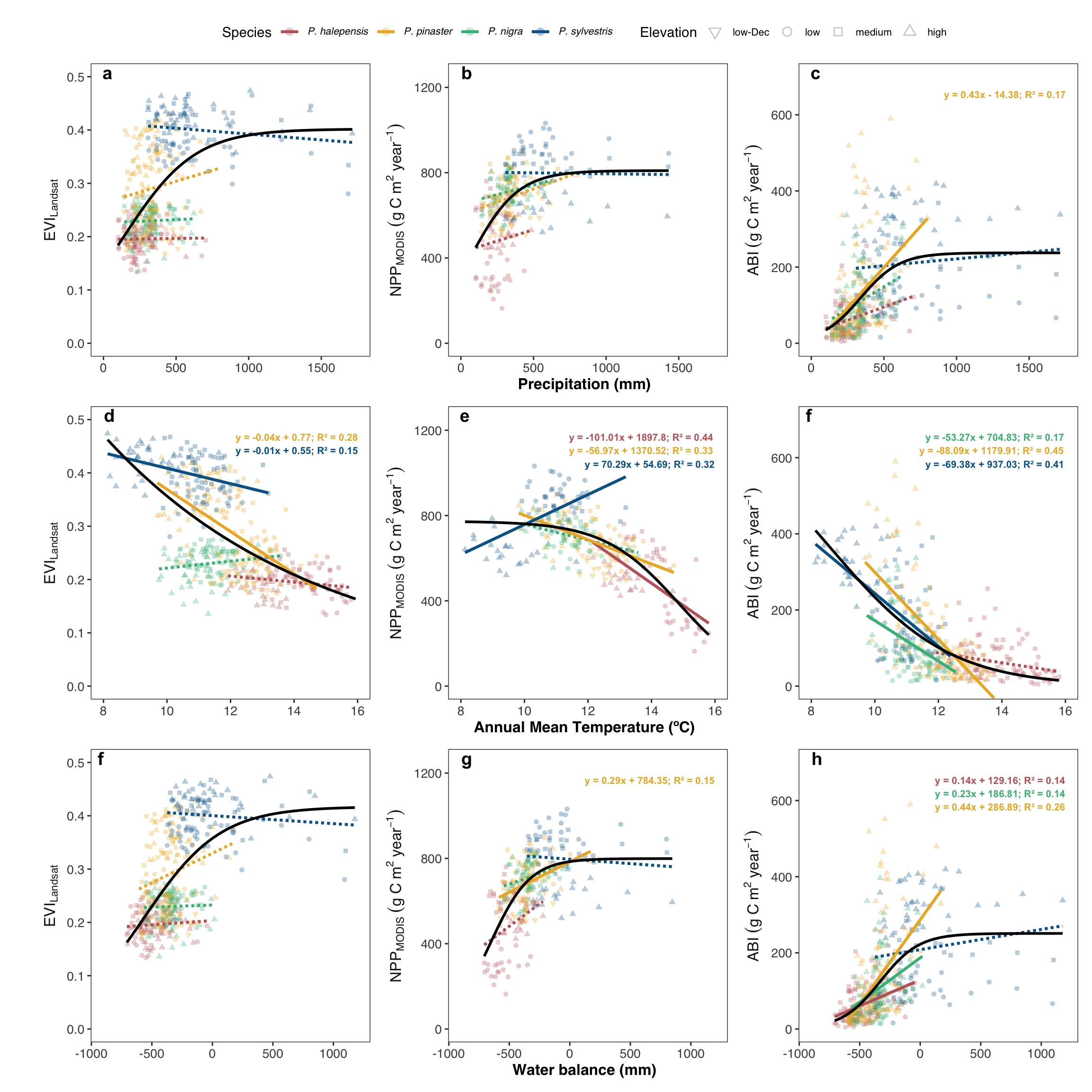
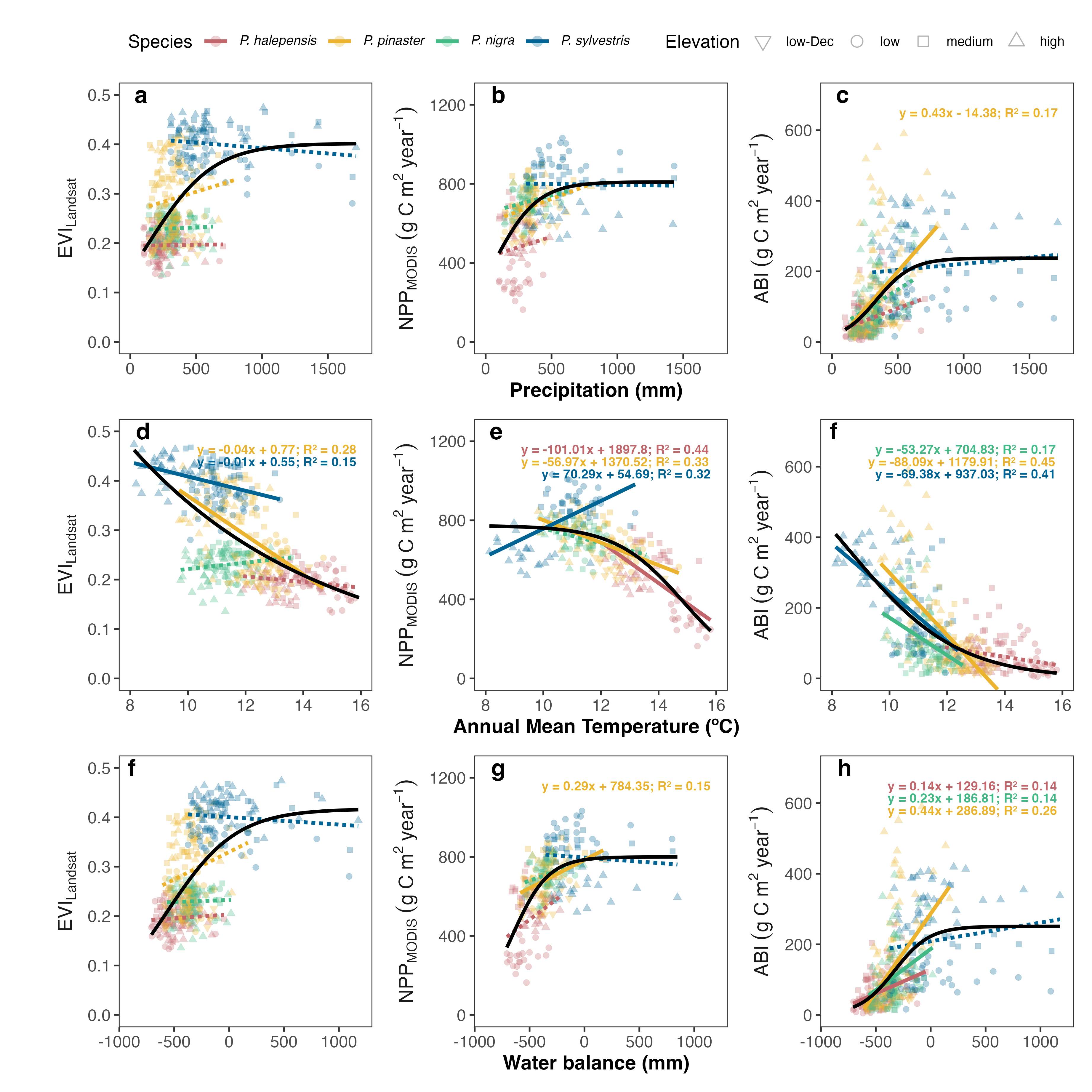
- This figure corresponds to figure 2 in the manuscript.
- An high-resolution version of this figure is available [here](../output/plot_combined_wb_prec_tmed.png).
```{r}
#| code-fold: true
#| fig-cap: "Relationships between annual Enhanced Vegetation Index (EVI) (1986-2022), annual Net Primary Productivity (NPP) (2001-2022), and Aboveground Biomass Increment (ABI) (1986-2022) with precipitation (a-c), annual mean temperature (d-f), and annual water balance (f-h). The global trends for all pine species are depicted by a black line (nonlinear least squares), while color-coded lines indicate relations for individual pine species (solid line: significant (p< 0.001), dashed line: not significant)."
#| fig-width: 12
#| fig-height: 12
# pkgs
library(tidyverse)
library(ggh4x)
library(patchwork)
library(here)
library(glue)
library(broom)
source(here::here("scripts/aux.R"))


# Read data
## ABI
abi <- read_csv(here::here("data/abi.csv")) |>
  mutate(se = NA, sd = NA, variable = "abi") |>
  rename(mean = abi)

## annual pet
annual_pet <- read_csv(here::here("data/spei_climate.csv")) |>
  dplyr::select(sp_elev, year, monthly_pet, monthly_tmed, monthly_prec) |>
  group_by(sp_elev, year) |>
  summarise(pet = sum(monthly_pet),
            prec = sum(monthly_prec),
            tmed = mean(monthly_tmed, na.rm = TRUE)) |>
  rowwise() |>
  mutate(water_balance = prec - pet)


## EVI Landsat
evi_landsat <- read_csv(here::here("data/iv_landsat.csv")) |>
  filter(iv == "evi") |>
  dplyr::select(year, sp_code, elev_code, sp_elev, mean, sd, se) |>
  mutate(variable = "evi_landsat")

## NPP MODIS
npp <- read_csv(here::here("data/npp_modis.csv")) |>
  rename(mean = npp) |>
  mutate(se = NA, sd = NA, variable = "npp") |>
  dplyr::select(year, sp_code, elev_code, sp_elev, mean, sd, se, variable)


df_index <- bind_rows(
  abi, evi_landsat, npp) |>
  mutate(elev_code = fct_relevel(elev_code, "low-Dec","low", "medium", "high")) |>
  mutate(Specie = paste0("P. ", sp_code)) |>
  rename(mean_y = mean, y_variable = variable)

df <- df_index |>
  inner_join(annual_pet) |>
  pivot_longer(pet:water_balance, values_to = "mean_climate",
               names_to = "climate_variable")

df_plot <- df |>
  filter(year > 1986) |>
  mutate(y_variable2 = case_when(
    y_variable == "abi" ~ "ABI~(g~C~m^2~year^{-1})",
    y_variable == "evi_landsat" ~ "EVI[Landsat]",
    y_variable == "npp" ~"NPP[MODIS]~(g~C~m^2~year^{-1})")) |>
  mutate(y_variable2 = fct_relevel(y_variable2,
                                   "EVI[Landsat]",
                                   "NPP[MODIS]~(g~C~m^2~year^{-1})",
                                   "ABI~(g~C~m^2~year^{-1})"))


# Generate tibble with y max values. Caution, check there are equal to ylimits specified below for plot
ymax_panel <- tibble(
   y_variable = c("evi_landsat", "npp", "abi"),
   y_max = c(0.5, 1250, 700))

# Generate another tibble with linear regression
lr <- df_plot |>
  filter(climate_variable != "pet") |>
  group_by(y_variable, climate_variable, sp_code) |>
  group_modify(~ {
    # Ajusta el modelo
    mod <- lm(mean_y ~ mean_climate, data = .x)

    # Tidy con coeficientes
    tidy_df <- broom::tidy(mod)

    # Añade R2 a cada fila
    tidy_df$r.squared <- broom::glance(mod)$r.squared

    tidy_df
  }) |>
  mutate(p = case_when(
    p.value < 0.001 ~ "<0.001",
    p.value >= 0.001 ~ as.character(round(p.value, 3))
  )) |>
  mutate(sig = case_when(
    p.value < 0.001 ~ "sig",
    p.value >= 0.001 ~ "no sig"
  ))

# Generate equations
l <- lr |>
  left_join(
    lr |> filter(term == "(Intercept)") |>
      select(y_variable, climate_variable, sp_code, intercept = estimate),
    by = c("y_variable", "climate_variable", "sp_code")
  ) |>
  mutate(
    eq_text = if_else(
      sig == "sig" & term == "mean_climate",
      glue("y = {round(estimate, 2)}x {ifelse(intercept < 0, '-', '+')} {round(abs(intercept), 2)}; R² = {round(r.squared, 2)}"),
     NA
    )
  ) |>
  filter(term != "(Intercept)") |>
  mutate(Specie = paste0("P. ", sp_code)) |>
  mutate(y_variable2 = case_when(
    y_variable == "evi_landsat" ~ "EVI[Landsat]",
    y_variable == "npp" ~ "NPP[MODIS]~(g~C~m^2~year^{-1})",
    y_variable == "abi" ~ "ABI~(g~C~m^2~year^{-1})"
  ))

# Filter equations
l_eq <- l |> filter(!is.na(eq_text)) |>
  left_join(ymax_panel, by = "y_variable") |>
  group_by(y_variable, climate_variable) |>
  mutate(
    offset_y = row_number() * 0.05 * y_max,  # Ajusta el offset según sea necesario
    y = y_max - offset_y
  ) |>
  ungroup()


df_plot <-
  df_plot |> left_join(
    l |> dplyr::select(y_variable, climate_variable, sp_code, p, sig)) |>
  mutate(sp_code = fct_relevel(sp_code, "halepensis","pinaster", "nigra", "sylvestris")) |>
  mutate(Specie = fct_relevel(Specie, "P. halepensis","P. pinaster", "P. nigra", "P. sylvestris"))


# Plot
## general_parameters

alpha_points <- 0.3
main_line_width <- 1
main_line_color <- "black"
partial_lines_width <- 1.1
size_points <- 1.7
stroke_points <- 0.1

label_landsat <- "EVI[Landsat]"
label_npp <- "NPP[MODIS]~(g~C~m^2~year^{-1})"
label_abi <- "ABI~(g~C~m^2~year^{-1})"
label_wb <- "P-PET (mm)"
label_prec <- "Precipitation (mm)"

y_scales <- list(
  scale_y_continuous(limits = c(0, 0.5)),
  scale_y_continuous(limits = c(0,1250)),
  scale_y_continuous(limits = c(0, 700))
)

## Custom themes
custom_scales <- list(
  scale_colour_manual(
    values = colours_Specie,
    labels = expression(italic("P. halepensis"), italic("P. pinaster"), italic("P. nigra"), italic("P. sylvestris")),
    name = "Species"),
  scale_fill_manual(
    values = colours_Specie,
    labels = expression(italic("P. halepensis"), italic("P. pinaster"), italic("P. nigra"), italic("P. sylvestris")),
    name = "Species"),
  scale_shape_manual(values = shape_elev, name = "Elevation")
)

base_theme <- list(
  theme_bw(),
  theme(text = element_text(family = "Helvetica"),
        axis.title.x = element_text(face = "bold", size = 12),
        strip.text = element_text(face = "bold", size = 12),
        axis.text = element_text(size = 10),
        legend.text = element_text(size = 8))
)

custom_theme_figure <- list(
  theme(
    panel.grid = element_blank(),
    strip.background = element_blank(),
    strip.placement = "outside",
    strip.text.y = element_text(vjust = 0)
  )
)


## Letters for label
letras <- data.frame(
  tipo = rep(c("prec", "temp", "wb"), each = 3),
  y_variable2 = rep(
    c("EVI[Landsat]", "NPP[MODIS]~(g~C~m^2~year^{-1})", "ABI~(g~C~m^2~year^{-1})"),
    times = 3
  ),
  label = c("a", "b", "c", "d", "e", "f", "g", "h", "i"),
  x = -Inf,
  y = Inf
)


# ----------

plot_prec <-
  df_plot|>
  filter(climate_variable == "prec") |>
  ggplot(aes(x=mean_climate, y = mean_y, colour = Specie)) +
  geom_point(aes(shape = elev_code, fill = Specie),
             alpha = alpha_points, size = size_points, stroke = stroke_points) +
  geom_smooth(aes(linetype = sig), linewidth = partial_lines_width, method = "lm", se = FALSE) +
  scale_linetype_manual(values = lines_lm, guide = "none") +
  geom_smooth(aes(),
              method = "nls",
              formula=y~SSlogis(x, Asym, xmid, scal),
              se =  FALSE, # this is important
              linewidth = main_line_width, colour = main_line_color) +
  ylab("") +
  xlab("Precipitation (mm)") +
  custom_scales +
  base_theme +
  custom_theme_figure +
  theme(
    legend.position = "top"
    # legend.box = "vertical"
  ) +
  scale_x_continuous(limits = c(0, 1750)) +
  facet_wrap(~factor(y_variable2, c("EVI[Landsat]",
                                    "NPP[MODIS]~(g~C~m^2~year^{-1})",
                                    "ABI~(g~C~m^2~year^{-1})")),
             scales = "free_y",
             labeller = label_parsed,
             strip.position = "left") +
  ggh4x::facetted_pos_scales(y = y_scales) +
  geom_text(data = (letras |> filter(tipo == "prec")),
            aes(x = x, y = y, label = label),
            vjust = 1.2, hjust = -1.2, size = 5,
            fontface = "bold", inherit.aes = FALSE) +
  geom_text(data = l_eq |> filter(climate_variable == "prec"),
            aes(x = Inf, y = y, label = eq_text),
            hjust = 1.1, vjust = 1.1, size = 2.75,
            fontface = "bold", show.legend = FALSE) +
  guides(
    colour = guide_legend(override.aes = list(size = 4)),
    shape = guide_legend(override.aes = list(size = 4)),
  )


# Add NLS for EVI and Temperature (not converge with nls general)

df_plot_tmed_evi <- df_plot |> filter(y_variable == "evi_landsat", climate_variable == "tmed")
nls_fit <- nls(mean_y ~ a * exp(-b * mean_climate) + c,
               start = list(
                 a = max(df_plot_tmed_evi$mean_y) - min(df_plot_tmed_evi$mean_y),
                 b = 0.1,
                 c = min(df_plot_tmed_evi$mean_y)
               ),
               data = df_plot_tmed_evi,
               control = nls.control(maxiter = 10000, tol = 1e-5, minFactor = 1e-7))

df_pred_tmed_evi <- data.frame(
  mean_climate =
    seq(min(df_plot_tmed_evi$mean_climate), max(df_plot_tmed_evi$mean_climate),
      length.out = 100
    )
) |>
  mutate(y_variable = "evi_landsat", climate_variable = "tmed") |>
  mutate(y_variable2 = "EVI[Landsat]")

df_pred_tmed_evi$mean_y <- predict(nls_fit, newdata = df_pred_tmed_evi)


df_pred_tmed_evi <- df_pred_tmed_evi |>
  bind_rows(
    data.frame(
      mean_climate = c(NA,NA),
      mean_y = c(NA,NA),
      y_variable = c("abi", "npp"),
      y_variable2 =
        c("NPP[MODIS]~(g~C~m^2~year^{-1})",
          "ABI~(g~C~m^2~year^{-1})"),
      climate_variable = c("tmed", "tmed")
    )
  )


plot_tmed <-
  df_plot |>
  filter(climate_variable == "tmed") |>
  ggplot(aes(x=mean_climate, y = mean_y, colour = Specie)) +
  geom_point(aes(shape = elev_code, fill = Specie),
             alpha = alpha_points, size = size_points, stroke = stroke_points) +
  geom_smooth(aes(linetype = sig), linewidth = partial_lines_width, method = "lm", se = FALSE) +
  scale_linetype_manual(values = lines_lm, guide = "none") +
  geom_smooth(
    data = df_plot |> filter(y_variable != "evi_landsat"),
    aes(),
              method = "nls",
              formula = y ~ SSlogis(x, Asym, xmid, scal),
              se =  FALSE, # this is important
              linewidth = main_line_width, colour = main_line_color) +
  ylab("") +
  xlab("Annual Mean Temperature (ºC)") +
  custom_scales +
  base_theme +
  custom_theme_figure +
  theme(
    legend.position = "none",
  ) +
  scale_x_continuous(limits = c(8, 16)) +
  facet_wrap(~factor(y_variable2, c("EVI[Landsat]",
                                    "NPP[MODIS]~(g~C~m^2~year^{-1})",
                                    "ABI~(g~C~m^2~year^{-1})")),
             scales = "free_y",
             labeller = label_parsed,
             strip.position = "left") +
  facetted_pos_scales(y = y_scales) +
  geom_text(data = (letras |> filter(tipo == "temp")),
            aes(x = x, y = y, label = label),
            vjust = 1.2, hjust = -1.2, size = 5,
            fontface = "bold", inherit.aes = FALSE) +
  geom_text(data = l_eq |> filter(climate_variable == "tmed"),
            aes(x = Inf, y = y, label = eq_text, colour = Specie),
            hjust = 1.1, vjust = 1.1, size = 2.75, inherit.aes = FALSE,
            fontface = "bold", show.legend = FALSE) +
  geom_line(data = df_pred_tmed_evi,
            aes(x = mean_climate, y = mean_y),
            linewidth = main_line_width,
            colour = main_line_color)

plot_wb <-
  df_plot|>
  filter(climate_variable == "water_balance") |>
  ggplot(aes(x=mean_climate, y = mean_y, colour = Specie)) +
  geom_point(aes(shape = elev_code, fill = Specie), alpha = alpha_points, size = size_points, stroke = stroke_points) +
  geom_smooth(aes(linetype = sig), linewidth = partial_lines_width, method = "lm", se = FALSE) +
  scale_linetype_manual(values = lines_lm, guide = "none") +
  geom_smooth(aes(),
              method = "nls",
              formula=y~SSlogis(x, Asym, xmid, scal),
              se =  FALSE, # this is important
              linewidth = main_line_width, colour = main_line_color) +
  ylab("") +
  xlab("Water balance (mm)") +
  custom_scales +
  base_theme +
  custom_theme_figure +
  theme(
    legend.position = "none",
  ) +
  scale_x_continuous(limits = c(-900, 1200)) +
  facet_wrap(~factor(y_variable2, c("EVI[Landsat]",
                                    "NPP[MODIS]~(g~C~m^2~year^{-1})",
                                    "ABI~(g~C~m^2~year^{-1})")),
             scales = "free_y",
             labeller = label_parsed,
             strip.position = "left") +
  facetted_pos_scales(y = y_scales) +
  geom_text(data = (letras |> filter(tipo == "wb")),
            aes(x = x, y = y, label = label),
            vjust = 1.2, hjust = -1.2, size = 5,
            fontface = "bold", inherit.aes = FALSE) +
  geom_text(data = l_eq |> filter(climate_variable == "water_balance"),
            aes(x = Inf, y = y, label = eq_text, colour = Specie),
            hjust = 1.1, vjust = 1.1, size = 2.75, inherit.aes = FALSE,
            fontface = "bold", show.legend = FALSE)

wb_prec_tmed <- plot_prec / plot_tmed /plot_wb  &
  guides(
    fill = guide_legend(order = 1, override.aes = list(size = 3)),
    colour = guide_legend(order = 1),
    shape = guide_legend(override.aes = list(stroke = .5, size = 3, colour = "black")),
  )

wb_prec_tmed
```
```{r}
#| echo: false
ggsave(
wb_prec_tmed,
file = here::here("output/plot_combined_wb_prec_tmed.png"),
dpi = 400,
width = 7.09*1.3, height = 7.09*1.3
)
```