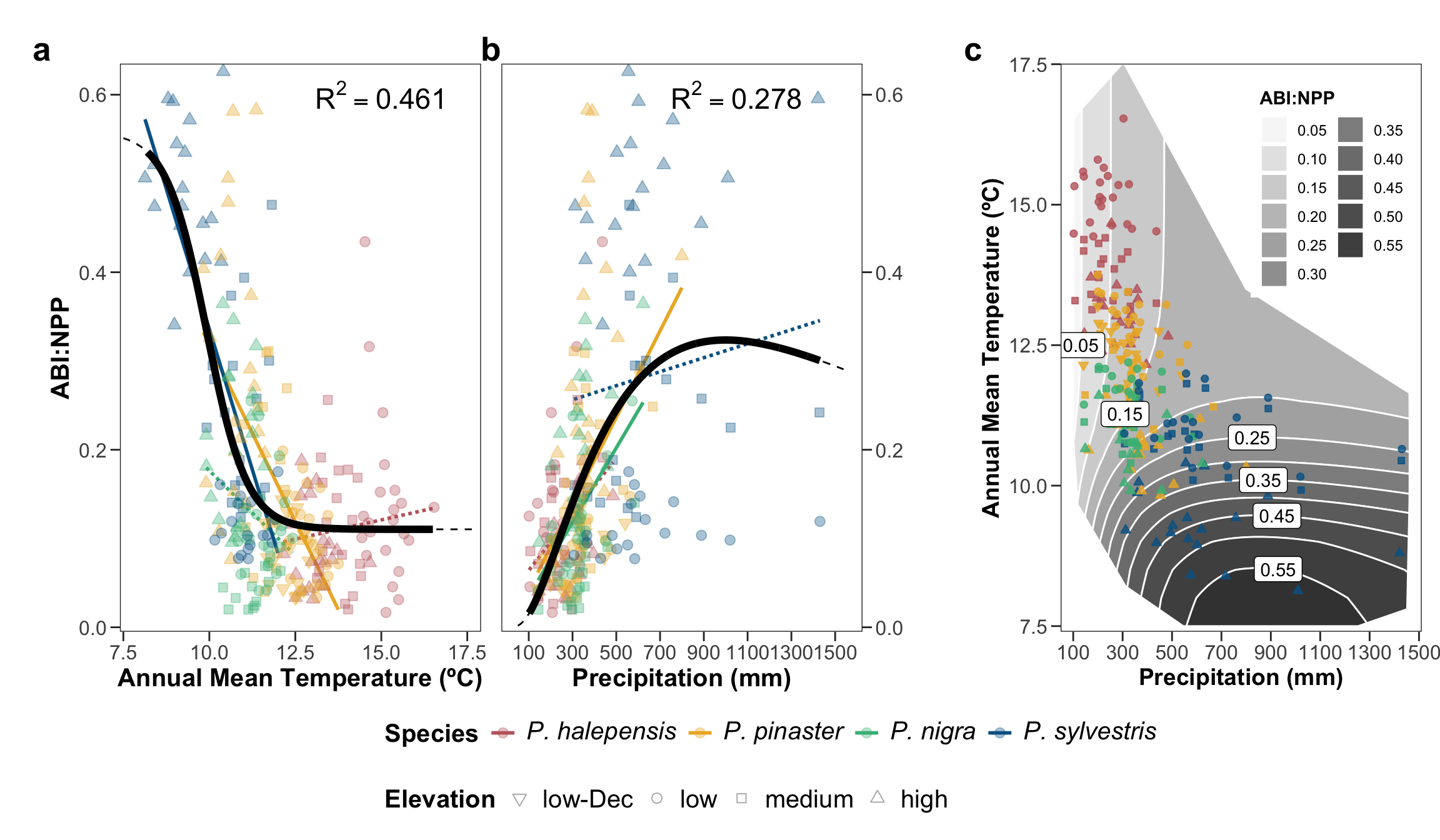
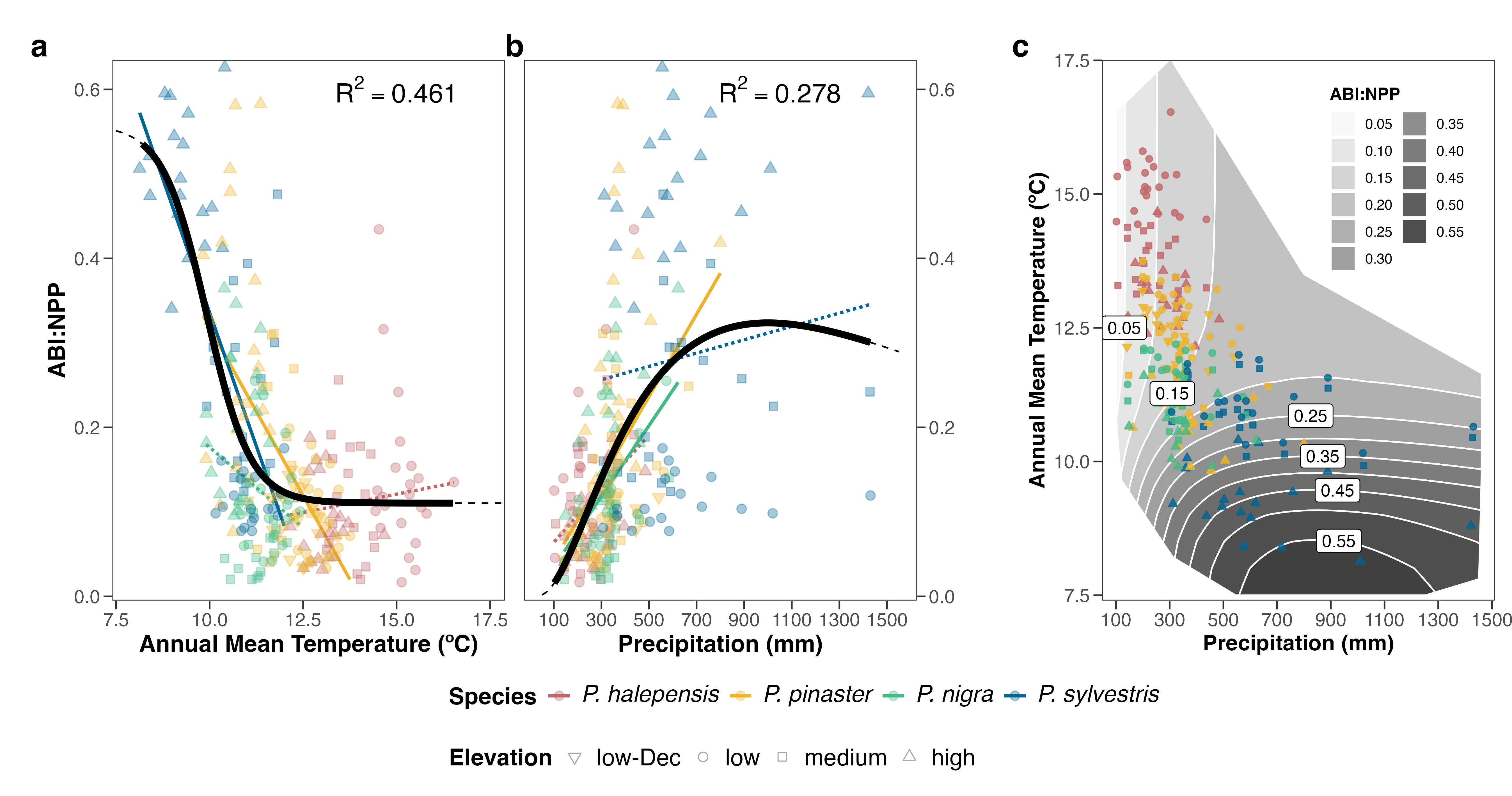
Relationships between ABI:NPP ratio and annual mean temperature (a) and precipitation (b). Nonlinear relationship between ABI:NPP ratio and climatic variables were shown by black solid lines (dashed black lines representing the relationships for unobserved climatic data). Color-coded lines indicate relations for individual pine species (solid line: significant (p<0.001), dashed line: not significant). (c) Response surface of the ABI:NPP ratio as a function of annual mean temperature and precipitation.
Source Code
---title: "Model Ratio ABI:NPP selected"format: html: toc: falseexecute: message: false warning: false---- This figure corresponds to figure 3 in the manuscript.- An high-resolution version of this figure is available [here](../output/plot_model_selected.jpg).```{r}#| code-fold: true#| fig-cap: "Relationships between ABI:NPP ratio and annual mean temperature (a) and precipitation (b). Nonlinear relationship between ABI:NPP ratio and climatic variables were shown by black solid lines (dashed black lines representing the relationships for unobserved climatic data). Color-coded lines indicate relations for individual pine species (solid line: significant (p<0.001), dashed line: not significant). (c) Response surface of the ABI:NPP ratio as a function of annual mean temperature and precipitation."#| fig-width: 12#| fig-height: 7library(tidyverse)library(ggnewscale)library(patchwork)library(broom)library(metR) library(sf)source("../scripts/aux.R")# Read dataannual_pet <-read_csv("../data/spei_climate.csv") |> dplyr::select(sp_elev, year, monthly_pet, monthly_tmed, monthly_prec) |>group_by(sp_elev, year) |>summarise(pet =sum(monthly_pet), prec =sum(monthly_prec),tmed =mean(monthly_tmed, na.rm =TRUE)) |>rowwise() |>mutate(water_balance = prec - pet)ratio <-read_csv("../data/ratio_abinpp.csv") |> dplyr::select(year, sp_code, elev_code, sp_elev, ratio_abi_npp = ratio) df <- ratio |>inner_join(annual_pet) |>pivot_longer(pet:water_balance, values_to ="mean_climate", names_to ="climate_variable")d <- df |>filter(climate_variable %in%c("tmed", "prec")) |>pivot_wider(values_from = mean_climate, names_from = climate_variable) |> dplyr::rename(rat = ratio_abi_npp) |>mutate(species =paste0("P. ", sp_code)) |>mutate(elev_code =fct_relevel(elev_code, "low-Dec", "low", "medium", "high")) |>mutate(sp_code =fct_relevel(sp_code, "halepensis","pinaster", "nigra", "sylvestris")) |>mutate(species =fct_relevel(species, "P. halepensis","P. pinaster", "P. nigra", "P. sylvestris")) # Read data from modelling # see modelling ratio selected.rmdteffect <-read_csv("../data/final_model_teffect.csv")peffect <-read_csv("../data/final_model_peffect.csv")pred_mcombrat7 <-read_csv("../data/final_model_pred_mcombrat7.csv")summary_models <-read_csv("../data/final_model_results.csv")#### Lineal models # For lineal models, response variable lm_temp <- d |>group_by(sp_code) |>group_modify(~ broom::tidy(lm(rat ~ tmed, data = .x)) ) |>filter(term !="(Intercept)") |>mutate(p =case_when( p.value <0.001~"<0.001", p.value >=0.001~as.character(round(p.value, 3)) )) |>mutate(sig =case_when( p.value <0.001~"sig", p.value >=0.001~"no sig" )) lm_prec <- d |>group_by(sp_code) |>group_modify(~ broom::tidy(lm(rat ~ prec, data = .x)) ) |>filter(term !="(Intercept)") |>mutate(p =case_when( p.value <0.001~"<0.001", p.value >=0.001~as.character(round(p.value, 3)) )) |>mutate(sig =case_when( p.value <0.001~"sig", p.value >=0.001~"no sig" )) # Plots parameters line_colour_model <-"black"alpha_points <-0.35size_points <-2.5label_npp <-"Annual~NPP[MODIS]~(g~C~m^2~year^{-1})"label_ratio <-"ABI:NPP"label_prec <-"Precipitation (mm)"label_tmed <-"Annual Mean Temperature (ºC)"label_wb <-"Water Balance (mm)"custom_options <-list(scale_shape_manual(values = shape_elev, name ="Elevation"), scale_colour_manual(values = colours_Specie, labels =expression(italic("P. halepensis"), italic("P. pinaster"), italic("P. nigra"), italic("P. sylvestris")),name ="Species"),scale_fill_manual(values = colours_Specie, labels =expression(italic("P. halepensis"), italic("P. pinaster"), italic("P. nigra"), italic("P. sylvestris")),name ="Species"),theme_bw(),theme(panel.grid =element_blank(), axis.title =element_text(size =15, face ="bold"), axis.text =element_text(size =12),axis.ticks.length =unit(.2, "cm"),legend.title=element_text(size=15, face ="bold"), legend.text=element_text(size=15) ))plot_t <- teffect |>filter(type_value =="predicted") |>filter(modelo =="mtrat6") |>ggplot(aes(x = tmed, y = value)) +# lineal geom_smooth(data = (d |>inner_join(lm_temp |> dplyr::select(sp_code, p, sig))),aes(x = tmed, y = rat, fill = species, colour = species, linetype = sig),linewidth =1, method ="lm", se =FALSE) +scale_linetype_manual(values = lines_lm, guide ="none") +geom_line(linetype ="dashed",colour = line_colour_model) +geom_point(data = d, aes(x = tmed, y = rat, shape = elev_code, fill = species, colour = species), alpha = alpha_points, size = size_points) +geom_line(data = (teffect |>filter(type_value =="predicted") |>filter(modelo =="mtrat6") |>filter(tmed >min(d$tmed)) |>filter(tmed <max(d$tmed))),colour = line_colour_model, linewidth =2.1) +scale_y_continuous(limits =c(0,0.63), expand =expansion(add =c(0.005, 0.005))) +scale_x_continuous(limits =c(7.5,17.8), expand =expansion(add =c(0.1, 0.1)),breaks =seq(7.5, 17.5, 2.5)) +xlab(label_tmed) +ylab(label_ratio) + custom_options +annotate(geom="text", x=15, y=.6, label=sprintf("R^2 == %.3g",round(summary_models |>filter(modelo =="mtrat6") |> dplyr::select(R2), 3)), color="black",parse =TRUE, size =6)plot_p <- peffect |>filter(type_value =="predicted") |>ggplot(aes(x = prec, y = value)) +geom_smooth(data = (d |>inner_join(lm_prec |> dplyr::select(sp_code, p, sig))),aes(x = prec, y = rat, fill = species, colour = species, linetype = sig),linewidth =1, method ="lm", se =FALSE) +scale_linetype_manual(values = lines_lm, guide ="none") +geom_line(linetype ="dashed",colour = line_colour_model) +geom_point(data = d, aes(x = prec, y = rat, shape = elev_code, fill = species, colour = species), alpha = alpha_points, size = size_points) +geom_line(data = (peffect |>filter(type_value =="predicted") |>filter(prec >min(d$prec)) |>filter(prec <max(d$prec))), colour = line_colour_model, linewidth =2.1) +scale_y_continuous(limits =c(0,0.63), expand =expansion(add =c(0.005, 0.005)), position ="right") +scale_x_continuous(limits =c(50, 1550), breaks =c(100, 300, 500, 700, 900, 1100, 1300, 1500)) +xlab(label_prec) +ylab("") + custom_options +annotate(geom="text", x=1050, y=.6, label =sprintf("R^2 == %.3g",round(summary_models |>filter(modelo =="mprecrat3") |> dplyr::select(R2), 3)), color="black",parse =TRUE, size =6) # Surface plotbreaks <-seq(0, .8, by=0.05)# Generate clip x <- d[chull(d$tmed, d$prec), c("rat","prec","tmed")] |>add_row(rat =0.075, prec =800, tmed =12.5) |>mutate(prec =ifelse(prec <150, prec -30, ifelse(prec >1300, prec +30, prec)))bb <-st_as_sf(x = x, coords =c("prec","tmed"), remove =FALSE) |>rename(ratio_pred = rat) |>st_combine() |>st_cast("POLYGON") |>st_buffer(dist =1)plot_with_ABI_legend <- pred_mcombrat7 |>ggplot(aes(x = prec, y = tmed)) +# Surface metR::geom_contour_fill(aes(z = ratio_pred, fill =after_stat(level)), binwidth =0.1,show.legend =TRUE, breaks = breaks, colour ="white", clip = bb) +# Colour scale surfacescale_fill_discretised(name = label_ratio, low ="#f7f7f7", high ="#404040", guide =guide_legend(override.aes =list(shape =NA), theme =theme(legend.title =element_text(size =11, face ="bold"),legend.text =element_text(size =9)), ncol =2 )) +theme_bw() +theme(panel.grid =element_blank(), axis.title =element_text(size =14, face ="bold"), axis.text =element_text(size =12),axis.ticks.length =unit(.2, "cm"),legend.position =c(0.75, 0.78) ) +# Add new scales ggnewscale::new_scale_color() + ggnewscale::new_scale_fill() +geom_point(data = d, aes(shape = elev_code, colour = species, fill = species), size =1.7, alpha = .8, show.legend =FALSE) +scale_shape_manual(values = shape_elev, name ="Elevation", guide ="none") +scale_colour_manual(values = colours_Specie, name ="Species", labels =expression(italic("P. halepensis"), italic("P. pinaster"), italic("P. nigra"), italic("P. sylvestris")),guide ="none") +scale_fill_manual(values = colours_Specie, name ="Species", labels =expression(italic("P. halepensis"), italic("P. pinaster"), italic("P. nigra"), italic("P. sylvestris")),guide ="none") + metR::geom_label_contour(aes(z = ratio_pred),colour ="black", breaks = breaks, label.placer =label_placer_n(n =1)) +xlab(label_prec) +ylab(label_tmed) +scale_y_continuous(limits =c(7.5, 17.5), breaks =c(7.5, 10, 12.5, 15, 17.5),expand =expansion(add =c(0.1, 0.01)) ) +scale_x_continuous(limits =c(50, 1510), breaks =c(100, 300, 500, 700, 900, 1100, 1300, 1500),expand =expansion(add =c(1, 1)) )main_figure2 <- ( (plot_t +theme(plot.margin =unit(c(0.5, 0, 0, .5), "cm")) + plot_p +theme(plot.margin =unit(c(0.5, .5, 0, 0), "cm")) &theme(legend.position ="bottom",legend.box ="vertical",legend.box.just ="left" )) +plot_layout(guides ="collect")+ (plot_with_ABI_legend +plot_layout(guides ="keep"))) +plot_annotation(tag_levels ="a") &theme(plot.tag =element_text(size =20, face ="bold"))main_figure2 ``````{r}#| echo: falseggsave( main_figure2, file ="../output/plot_model_selected.jpg",dpi =400,width =7.09*1.9, height =7.09)```