---
title: "Time series of EVI, NPP, ABI and ABI:NPP ratio"
format:
html:
toc: false
execute:
message: false
warning: false
---
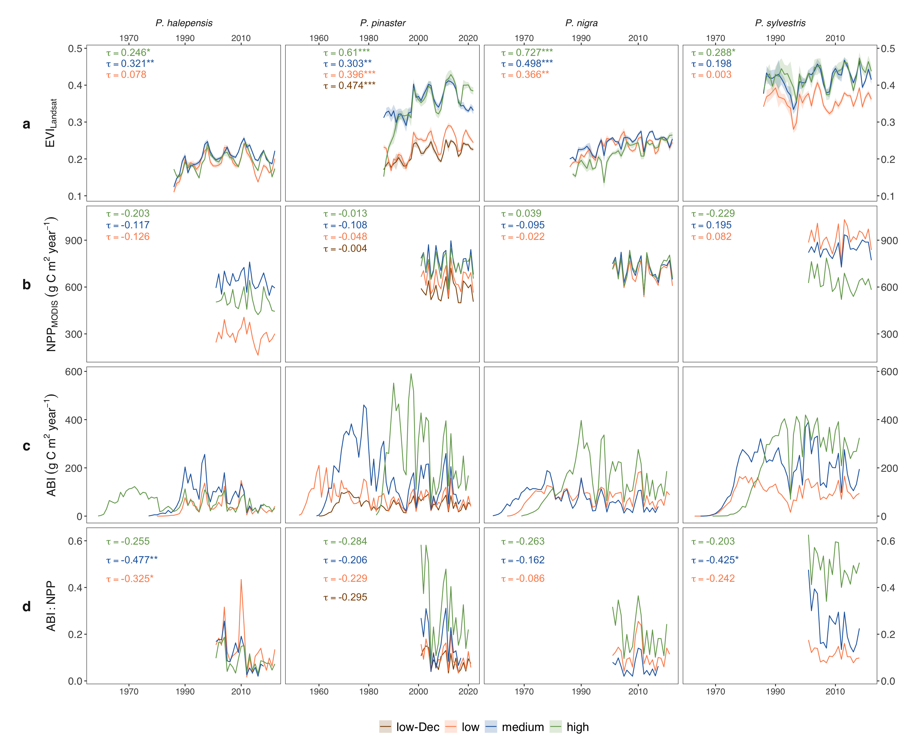
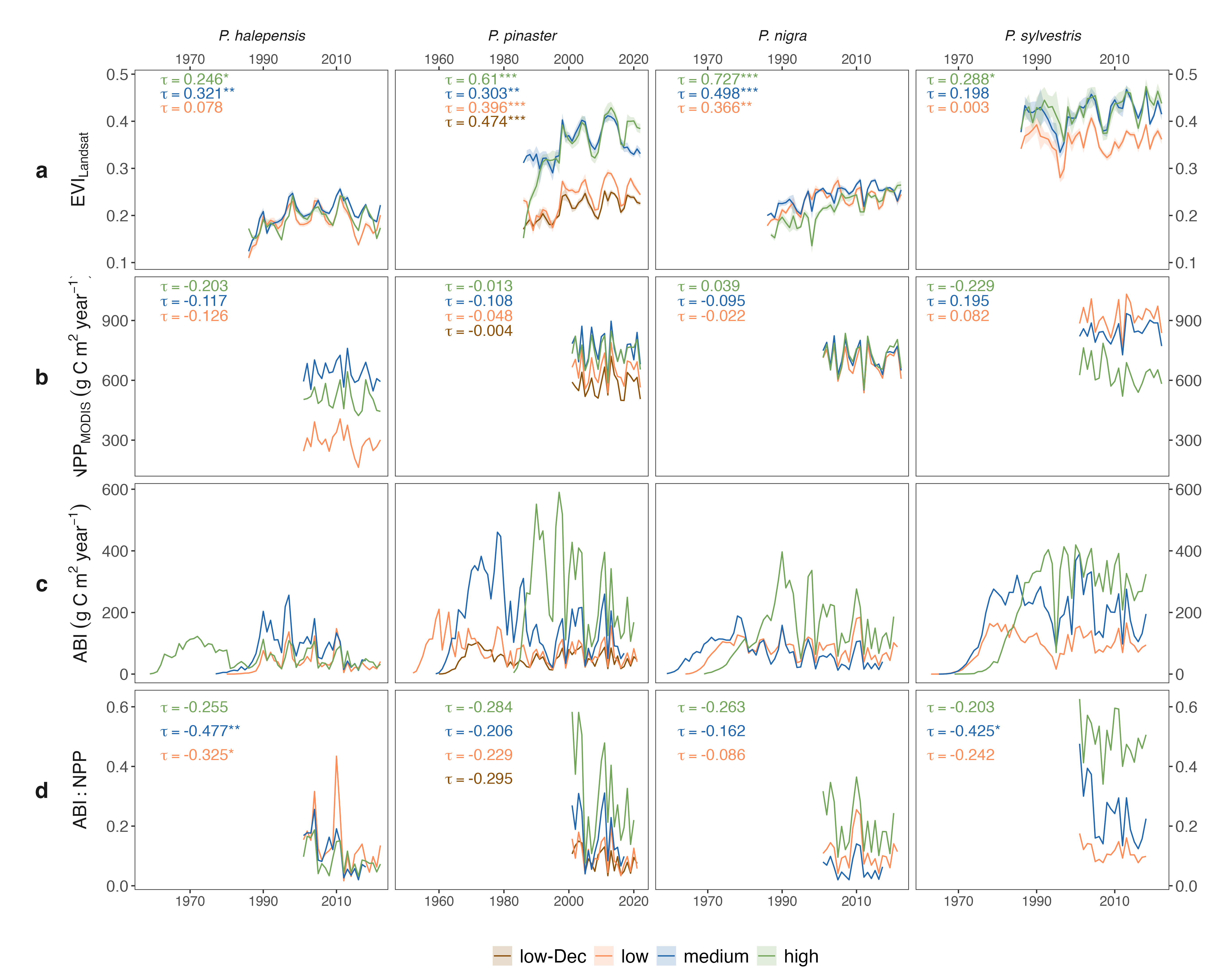
- This figure corresponds to figure S5 in the manuscript.
- An high-resolution version of this figure is available [here](../output/plot_ts_dendro_remote.jpg).
```{r}
#| code-fold: true
#| fig-cap: "Time series of annual Enhanced Vegetation Index (EVI) (1986-2022) (a), annual Net Primary Productivity (NPP) (2001-2022) (b), Aboveground Biomass Increment (ABI) (1952-2022) (c), and ABI:NPP ratio (2001-2022) (d). Within each species, each line represents the temporal series for different elevation sites, distinguished by different colors. For annual EVI, ribbons represent the standard error of the annual values. Mann-Kendall tau values indicated were computed for each temporal series starting from 1986 for EVI and from 2001 for NPP and ABI:NPP ratio. Significant values of the trends are indicated: * p-value < 0.05; ** p-value < 0.01; *** p-value < 0.001."
#| fig-width: 16
#| fig-height: 13
library(tidyverse)
library(kableExtra)
library(ggh4x)
library(Kendall)
library(trend)
source("../scripts/aux.R")

abi <- read_csv("../data/abi.csv") |>
  mutate(se = NA, sd = NA, variable = "abi") |>
  rename(mean = abi)

npp <- read_csv("../data/npp_modis.csv") |>
  rename(mean = npp) |>
  mutate(se = NA, sd = NA, variable = "npp") |>
  dplyr::select(year, sp_code, elev_code, sp_elev, mean, sd, se, variable)

evi_landsat <- read_csv("../data/iv_landsat.csv") |>
  filter(iv == "evi") |>
  dplyr::select(year, sp_code, elev_code, mean, sd, se) |>
  mutate(variable = "evi_landsat")

ratio <- read_csv("../data/ratio_abinpp.csv") |>
  dplyr::select(year, sp_code, elev_code, sp_elev, mean = ratio) |>
  mutate(se = NA, sd = NA, variable = "ratio")


df <- bind_rows(
  abi, evi_landsat, npp, ratio) |>
  # mutate(elev_code = fct_recode(elev_code, `low-Dec` = "low2")) |>
  mutate(elev_code = fct_relevel(elev_code, "low-Dec","low", "medium", "high")) |>
  mutate(Specie = paste0("P. ", sp_code))


# Import data trends
mk_evi_landsat <- read_csv("../data/iv_landsat_trend.csv") |>
  dplyr::select(sp_code, elev_code, sp_elev, tau = mean_tau, pvalue_mk = mean_pvalue_mk,  senslope = mean_senslope, pvalue_sen= mean_pvalue_sen, ypos, p_value_string, taulabel) |>
  mutate(variable = "evi_landsat")

mk_npp <- read_csv("../data/npp_modis_trend.csv") |>
  rename(tau = npp_tau,
         pvalue_mk = npp_pvalue_mk,
         senslope = npp_senslope,
         pvalue_sen = npp_pvalue_sen) |>
  mutate(variable = "npp") |>
  mutate(ypos2 = case_when(
    ypos == 1000 ~ 850,
    ypos == 1025 ~ 925,
    ypos == 1050 ~ 1000,
    ypos == 1075 ~ 1075)) |>
  dplyr::select(-ypos, -Specie) |> rename(ypos = ypos2) |>
  mutate(p_value_string = as.character(p_value_string))

mk_abi <- read_csv("../data/abi_trend.csv") |>
  rename(tau = mean_tau,
         pvalue_mk = mean_pvalue_mk,
         senslope = mean_senslope,
         pvalue_sen = mean_pvalue_sen) |>
  mutate(variable = "abi") |>
  mutate(ypos2 = case_when(
    ypos == 510 ~ 480,
    ypos == 540 ~ 525,
    ypos == 570 ~ 570,
    ypos == 480 ~ 435)) |>
  dplyr::select(-ypos, -Specie) |> rename(ypos = ypos2) |>
  mutate(p_value_string = as.character(p_value_string))


mk_ratio <- ratio |>
  ungroup() |>
  group_by(sp_code, elev_code, sp_elev)|>
  summarise(across(c(mean), ~MannKendall(.)$tau, .names ="tau"),
            across(c(mean), ~MannKendall(.)$sl, .names ="pvalue_mk"),
            across(c(mean), ~trend::sens.slope(.)$estimate, .names ="senslope"),
            across(c(mean), ~trend::sens.slope(.)$p.value, .names ="pvalue_sen")) |>
  mutate(ypos =
           case_when(
             elev_code == "low" ~ .44,
             elev_code == "low-Dec" ~ .36,
             elev_code == "medium" ~ .52,
             elev_code == "high" ~ .6),
         p_value_string = as.character(symnum(pvalue_mk, corr = FALSE,
                                              cutpoints = c(0,  .001,.01,.05, 1),
                                              symbols = c("***","**","*",""))),
         variable = "ratio") |>
  mutate(taulabel = paste(expression(tau), "==", paste0('"', round(tau, 3), p_value_string, '"'))) |>
  mutate(
    Specie = paste0("P. ", sp_code)
  ) |>
  mutate(taulabel = gsub("-", "\U2212", taulabel))


mk <- bind_rows(mk_evi_landsat, mk_npp, mk_abi, mk_ratio) |>
  mutate(variable = fct_relevel(variable, "evi_landsat", "npp", "abi", "ratio")) |>
  # mutate(elev_code = fct_recode(elev_code, `low-Dec` = "low2")) |>
  mutate(elev_code = fct_relevel(elev_code, "low-Dec","low", "medium", "high")) |>
  mutate(Specie = paste0("P. ", sp_code))

# replace minus sign in taulabel (−) by unicode
mk$taulabel <- gsub("−", "-", mk$taulabel)


to_label <- as_labeller(c(
  "evi_landsat" = "EVI[Landsat]",
  "npp" = "NPP[MODIS]~(g~C~m^2~year^{-1})",
  "abi" = "ABI~(g~C~m^2~year^{-1})",
  "ratio" = "ABI:NPP"
), default = label_parsed)


### To add letters to the facet
label_rows <- data.frame(
  variable = c("evi_landsat", "npp", "abi", "ratio"),
  letra = c("a", "b", "c", "d")
)

df <- df |> inner_join(label_rows)
mk <- mk |> inner_join(label_rows)

fig_ts <- df |>
  filter(variable != "evi_modis") |>
  mutate(variable = fct_relevel(variable, "evi_landsat", "npp", "abi", "ratio")) |>
  mutate(elev_code = fct_relevel(elev_code, "low-Dec","low", "medium", "high")) |>
  ggplot(aes(x = year, y = mean, group = elev_code, colour = elev_code)) +
  geom_ribbon(aes(ymin = (mean - se), ymax=(mean+se), fill=elev_code), colour=NA, alpha=.2) +
  geom_line() +
  ggh4x::facet_nested(letra + variable ~factor(Specie, levels = c("P. halepensis", "P. pinaster", "P. nigra", "P. sylvestris")),
               scales = "free",
               switch = "y",
               labeller = labeller(variable = to_label),
               strip = ggh4x::strip_themed(
                 text_y = list(
                   element_text(face = "bold", size = 18, angle = 0),
                   element_text(face = "bold", size = 18, angle = 0),
                   element_text(face = "bold", size = 18, angle = 0),
                   element_text(face = "bold", size = 18, angle = 0),
                   element_text(face = "bold", size = 15),
                   element_text(face = "bold", size = 15),
                   element_text(face = "bold", size = 15),
                   element_text(face = "bold", size = 15)
                   ))) +
  scale_colour_manual(values = colours_elev2, name = "") +
  scale_fill_manual(values = colours_elev2, name="") +
  scale_y_continuous(sec.axis = dup_axis()) +
  geom_text(aes(x = min(df$year, na.rm = TRUE) + 5, y = ypos, label = taulabel),
            position = position_nudge(x = 5),
            data = (mk |> filter(variable != "abi")),
            parse = TRUE, show.legend = FALSE, hjust = "left", size = 4.5) +
  ggh4x::facetted_pos_scales(
  x = list(
    scale_x_continuous(limits = c(1958,2021), breaks = seq(1950, 2020, by = 20), minor_breaks = seq(1950, 2020, by = 10), guide = "axis_minor", sec.axis = dup_axis()), # halepensis
    scale_x_continuous(limits = c(1950,2021), breaks = seq(1940, 2020, by = 20), minor_breaks = seq(1950, 2020, by = 10), guide = "axis_minor", sec.axis = dup_axis()), # pinaster
    scale_x_continuous(limits = c(1959,2021), breaks = seq(1950, 2020, by = 20), minor_breaks = seq(1950, 2020, by = 10), guide = "axis_minor", sec.axis = dup_axis()), # nigra
    scale_x_continuous(limits = c(1962,2021), breaks = seq(1950, 2020, by = 20), minor_breaks = seq(1950, 2020, by = 10), guide = "axis_minor", sec.axis = dup_axis())  # pinaster
  )
) +
  theme_bw() +
  ylab("") +  xlab("") +
  theme(
    text = element_text(family = "Helvetica"),
    panel.grid = element_blank(),
    panel.background = element_blank(),
    strip.text.x = element_text(face = "italic", size = 12),
    strip.background = element_blank(),
    strip.placement = "outside",
    legend.position = "bottom",
    legend.text = element_text(size = 15),
    axis.text.y = element_text(size = 13),
    axis.text.x = element_text(size = 11),
    ggh4x.axis.ticks.length.minor = rel(1)
  )

fig_ts
```
```{r}
#| echo: false
ggsave(
fig_ts,
file = "../output/plot_ts_dendro_remote.jpg",
dpi = 400,
width = 7.09*1.3*1.5, height = 7.09*1.3*1.2
)
```