Prepara los datos de mariposas
Antonio J. Pérez-Luque
2021-12-28
Last updated: 2022-07-12
Checks: 7 0
Knit directory: ms_mariposas_biodiversity/
This reproducible R Markdown analysis was created with workflowr (version 1.7.0). The Checks tab describes the reproducibility checks that were applied when the results were created. The Past versions tab lists the development history.
Great! Since the R Markdown file has been committed to the Git repository, you know the exact version of the code that produced these results.
Great job! The global environment was empty. Objects defined in the global environment can affect the analysis in your R Markdown file in unknown ways. For reproduciblity it’s best to always run the code in an empty environment.
The command set.seed(20211228) was run prior to running
the code in the R Markdown file. Setting a seed ensures that any results
that rely on randomness, e.g. subsampling or permutations, are
reproducible.
Great job! Recording the operating system, R version, and package versions is critical for reproducibility.
Nice! There were no cached chunks for this analysis, so you can be confident that you successfully produced the results during this run.
Great job! Using relative paths to the files within your workflowr project makes it easier to run your code on other machines.
Great! You are using Git for version control. Tracking code development and connecting the code version to the results is critical for reproducibility.
The results in this page were generated with repository version 7ef7a0e. See the Past versions tab to see a history of the changes made to the R Markdown and HTML files.
Note that you need to be careful to ensure that all relevant files for
the analysis have been committed to Git prior to generating the results
(you can use wflow_publish or
wflow_git_commit). workflowr only checks the R Markdown
file, but you know if there are other scripts or data files that it
depends on. Below is the status of the Git repository when the results
were generated:
Ignored files:
    Ignored:    .Rhistory
    Ignored:    .Rproj.user/

Unstaged changes:
    Modified:   figs/plot_rarefaction.pdf
    Modified:   figs/plot_species_acumulation_area.pdf
Note that any generated files, e.g. HTML, png, CSS, etc., are not included in this status report because it is ok for generated content to have uncommitted changes.
These are the previous versions of the repository in which changes were
made to the R Markdown
(analysis/prepara_datos_mariposas.Rmd) and HTML
(docs/prepara_datos_mariposas.html) files. If you’ve
configured a remote Git repository (see ?wflow_git_remote),
click on the hyperlinks in the table below to view the files as they
were in that past version.
| File | Version | Author | Date | Message |
|---|---|---|---|---|
| Rmd | 7ef7a0e | ajpelu | 2022-07-12 | update |
| html | 9471064 | ajpelu | 2022-07-12 | Build site. |
| Rmd | 3f62ed0 | ajpelu | 2022-07-12 | rarefaction |
| html | f07aef2 | ajpelu | 2022-07-11 | update prepara datos. Add Species accumulation area |
| Rmd | 02d90ff | ajpelu | 2022-07-11 | datos nuevos modelos |
| html | 915669b | ajpelu | 2022-02-04 | Build site. |
| html | c814af8 | ajpelu | 2022-01-18 | fix error link ambientales |
| html | d441a65 | ajpelu | 2022-01-18 | Build site. |
| Rmd | e6ecd35 | ajpelu | 2022-01-18 | compute richness |
| html | cece0cb | ajpelu | 2022-01-18 | Build site. |
| Rmd | 2cf9d33 | ajpelu | 2022-01-18 | quita transectos Cáñar, HoyaMora |
| html | a4134b0 | ajpelu | 2021-12-30 | Build site. |
| Rmd | ec59e79 | ajpelu | 2021-12-30 | Generate script of prepara datos |
Introduction
En este apartado usamos los datos de contactos de mariposas para su preparación.
library(tidyverse)
library(readxl)
library(janitor)
library(here)
library(lubridate)
library(DT)
library(vegan)
library(writexl)
library(iNEXT)
Preparación de datos
Usamos datos descargados directamente de linaria.obsnev.es. Tenemos dos archivos: conteos y visitas.
Utilizamos solo fecha de inicio y computamos mes, año y día de cada contacto.
Filtramos los datos:
- No utilizaremos los años 2008, 2009, 2010, 2011, 2021
- No utilizaremos datos de los meses de marzo, abril, septiembre y octubre
- No usamos los datos: Robledal de Cáñar ni Hoya de la Mora
rawdata <- read_delim(here::here("data/mariposas_diurnas_contactos_transectos.csv"), delim = ";") %>%
  janitor::clean_names() %>%
  mutate(year = lubridate::year(fecha_inicio),
         month = lubridate::month(fecha_inicio),
         day = lubridate::day(fecha_inicio)) %>%
  dplyr::select(-fecha_fin, -fecha_inicio)

d <- rawdata %>%
  filter(year >= 2011) %>%
  filter(year < 2021) %>%
  filter(!(month %in% c(3,4,9,10))) %>%
  filter(transecto != "Hoya de la Mora") %>%
filter(transecto != "Robledal de Cáñar") - Leer información de transectos: longitud, abreviatura; y creamos una variable llamada elev (elevación) que corresponde al promedio entre la altura mínima y máxima del transecto.
metadata_transectos <- read_excel(here::here("data/longitud_transectos.xlsx"),
                 sheet = "Longitud_transectos") %>%
  janitor::clean_names() %>%
  mutate(id_transecto = paste0("16_",transectid))

abrev <- read_csv(here::here("data/transect_abrev.csv")) %>% janitor::clean_names() %>%
  rename(id_transecto = id_transect)

transectos <- metadata_transectos %>%
  inner_join(abrev) %>%
  dplyr::select(-transectid, -transect) %>%
  rowwise() %>%
  mutate(elev = round(((min_altitu+max_altitu)/2),0)) %>%
  rename(transecto = name)

write_csv(transectos, here::here("data/transectos_tabla.csv"))
Total contactos transecto y año
- Generamos un dataset con el total (número de contactos) por transecto y visita
ntotal_transecto_visita <- d %>%
  group_by(id_visita, id_transecto, transecto, year) %>%
summarise(ntotal = sum(total)) - Leemos información de las visitas realizadas a los transectos. Genero un dataset de visitas con aquellas visitas sin contactos
rawvisitas <- read_delim(here::here("data/mariposas_diurnas_visitas.csv"),
                      delim = ";", col_types = cols(Temperatura = col_number())) %>% janitor::clean_names() %>%
    mutate(year = lubridate::year(fecha_inicio),
         month = lubridate::month(fecha_inicio),
         day = lubridate::day(fecha_inicio)) %>%
  dplyr::select(-fecha_fin, -fecha_inicio)

visitas <- rawvisitas %>%
  filter(year >= 2011) %>%
  filter(year < 2021) %>%
  filter(transecto_parcela != "Hoya de la Mora") %>%
  filter(transecto_parcela != "Robledal de Cáñar") %>%
  filter(!(month %in% c(3,4,9,10))) %>%
  dplyr::select(id_visita=id, transecto=transecto_parcela, year, month, day)

ntotal_transecto_visitas_cero <- visitas %>%
  filter(!(id_visita %in% unique(d$id_visita))) %>%
  mutate(ntotal = 0) %>%
  dplyr::select(-month, -day) %>%
  inner_join((transectos %>% dplyr::select(transecto, id_transecto))) %>%
  relocate(id_visita, transecto, id_transecto)
Unimos los dos datasets anteriores y le adjuntamos información de los transectos.
Filtramos los datos de 2018. Eliminamos todas las visitas de 2018 excepto para los transectos Pitres, Dúrcal, Turbera, Laguna (“16_45”,“16_46”,“16_48”,“16_49”)
ntotalraw <- bind_rows(ntotal_transecto_visita, ntotal_transecto_visitas_cero) %>% inner_join(transectos)

ntotal <- ntotalraw %>%
  filter(!(year == 2018 & !id_transecto %in% c("16_45","16_46","16_48","16_49")))
Densidad
- Densidad por año
densidad_by_year <- ntotal %>%
  group_by(id_transecto, transecto, site, elev, year) %>%
  summarise(abundancia = sum(ntotal),
         long_total = sum(longitud) / 100) %>%
  mutate(den = abundancia / long_total)
write_csv(densidad_by_year, here::here("data/densidad_by_year.csv"))datatable(densidad_by_year)Diversidad
- ¿Cuantas especies se han contactado?. Observamos que hay registros de taxones identificados a diferentes niveles. Vamos a ver aquellos que estén registrados a nivel al menos específico.
taxones_anotados <- d %>%
  dplyr::select(id_especie, nombre_cientifico) %>% unique() %>%
  mutate(w = stringr::str_count(nombre_cientifico, "\\w+"))

especies <- taxones_anotados %>% filter(w>1)
m <- d %>%
filter(!(year == 2018 & !id_transecto %in% c("16_45","16_46","16_48","16_49"))) %>%
filter(nombre_cientifico %in% especies$nombre_cientifico) %>%
mutate(sp = stringr::word(nombre_cientifico, start = 1, end = 2)) %>%
mutate(spabrev = stringr::str_replace(sp," ", ".")) %>%
dplyr::select(-sp) %>%
mutate(sp = str_replace(spabrev, " ", ".")) %>%
group_by(transecto, spabrev, year) %>%
summarise(n_ind = sum(total)) %>%
pivot_wider(names_from = year,
values_from=n_ind,
names_prefix = "y", values_fill = 0) %>% as.data.frame()
years <- c("y2012","y2013","y2014","y2015","y2016","y2017","y2018","y2019","y2020")
out_h <- data.frame()
for (y in years){
vars <- c("spabrev", "transecto", y)
aux_diversidad <- m %>%
dplyr::select(all_of(vars)) %>%
pivot_wider(names_from = spabrev, values_from = y, values_fill = 0) %>%
column_to_rownames(var = "transecto")
h <- vegan::diversity(aux_diversidad) %>% as.data.frame()
names(h) <- "diversidad"
h$year <- y
h$transecto <- row.names(h)
out_h <- rbind(out_h, h)
}
# Ojo en el cómputo de diversidad aparecen años y transectos con 0. Creo que es un error. Los dejo con NA
rownames(out_h) <- NULL
diversidad <- out_h %>%
mutate(year = as.numeric(substring(year,2)),
diversidad = na_if(diversidad,0)) %>%
inner_join(transectos)
write_csv(diversidad, here::here("data/diversidad_by_year.csv"))datatable(diversidad)Riqueza
riq <- d %>%
  filter(!(year == 2018 & !id_transecto %in% c("16_45","16_46","16_48","16_49"))) %>%
  filter(nombre_cientifico %in% especies$nombre_cientifico) %>%
  mutate(sp = stringr::word(nombre_cientifico, start = 1, end = 2)) %>%
  mutate(spabrev = stringr::str_replace(sp," ", ".")) %>%
  dplyr::select(-sp) %>%
  group_by(transecto, year) %>%
  summarise(sp_unique = unique(spabrev)) %>%
  group_by(transecto, year) %>%
  count() %>%
  rename(riq = n) %>%
  inner_join(transectos)

write_csv(riq, here::here("data/riqueza_by_year.csv"))datatable(riq)riq_site <- d %>%
filter(!(year == 2018 & !id_transecto %in% c("16_45","16_46","16_48","16_49"))) %>%
filter(nombre_cientifico %in% especies$nombre_cientifico) %>%
mutate(sp = stringr::word(nombre_cientifico, start = 1, end = 2)) %>%
mutate(spabrev = stringr::str_replace(sp," ", ".")) %>%
dplyr::select(-sp) %>%
group_by(transecto) %>%
summarise(sp_unique = unique(spabrev)) %>%
group_by(transecto) %>%
count() %>%
rename(riq = n) %>%
inner_join(transectos)
write_csv(riq_site, here::here("data/riqueza_by_site.csv"))Tabla suplementaria especies - transectos
ts <- d %>%
  filter(!(year == 2018 & !id_transecto %in% c("16_45","16_46","16_48","16_49"))) %>%
  filter(nombre_cientifico %in% especies$nombre_cientifico) %>%
  group_by(transecto, nombre_cientifico, year) %>%
  summarise(n_ind = sum(total)) %>%
  pivot_wider(names_from = year,
              values_from=n_ind,
              names_prefix = "y", values_fill = 0) %>% as.data.frame() %>%
  inner_join(transectos) %>%
  rowwise() %>%
  mutate(contactos = sum(across(starts_with("y")))) %>%
  mutate(n_years_contacted = 9 - sum(across(starts_with("y")) == 0)) # Número total de años (9) - años con cero contactos

write_csv(ts, here::here("data/tabla_especies_transectos.csv"))

tsall <- d %>%
  filter(!(year == 2018 & !id_transecto %in% c("16_45","16_46","16_48","16_49"))) %>%
  group_by(transecto, nombre_cientifico, year) %>%
  summarise(n_ind = sum(total)) %>%
  pivot_wider(names_from = year,
              values_from=n_ind,
              names_prefix = "y", values_fill = 0) %>% as.data.frame() %>%
  inner_join(transectos) %>%
  rowwise() %>%
  mutate(contactos = sum(across(starts_with("y")))) %>%
  mutate(n_years_contacted = 9 - sum(across(starts_with("y")) == 0))

write_csv(tsall, here::here("data/tabla_taxones_transectos.csv"))
Species accumulation curve
curvas_spec <- data.frame()

for (i in unique(m$transecto)) {
  aux <- m %>% filter(transecto==i) %>%
    relocate(y2018, .after=y2017) %>%
    ungroup() %>% dplyr::select(-transecto) %>%
    pivot_longer(-spabrev, names_to = "year", values_to = "nind") %>%
    pivot_wider(names_from = spabrev, values_from = nind) %>% column_to_rownames("year") %>%
    as.data.frame()

  sca <- vegan::specaccum(aux, method = "collector")

  sca_random <- vegan::specaccum(aux, method = "random", permutations = 499)

  s <- data.frame(richness = sca_random$richness,
                  sd = sca_random$sd,
                  sites = sca_random$sites,
                  richness_real = sca$richness,
                  years = seq(2012,2020,1))

  rownames(s) <- NULL
  s$transecto <- i

  curvas_spec <- rbind(curvas_spec, s)
}


plot_curvas <- curvas_spec %>%
  ggplot(aes(x=years, y=richness)) +
  theme_minimal() +
  geom_ribbon(aes(ymin = richness - 1.96*sd, ymax = richness + 1.96*sd), fill="lightblue", alpha =.5) +
  geom_line(colour = "blue") +
  geom_line(aes(y=richness_real), col = "black") +
  facet_wrap(~transecto, scales = "free_y", ncol = 4) +
  xlab('year') + ylab('Richness') +
  theme(panel.grid.minor = element_blank())
ggsave(here::here("figs/plot_species_acumulation_area.pdf"),
device = "pdf",
width = 12, height = 11)
plot_curvas 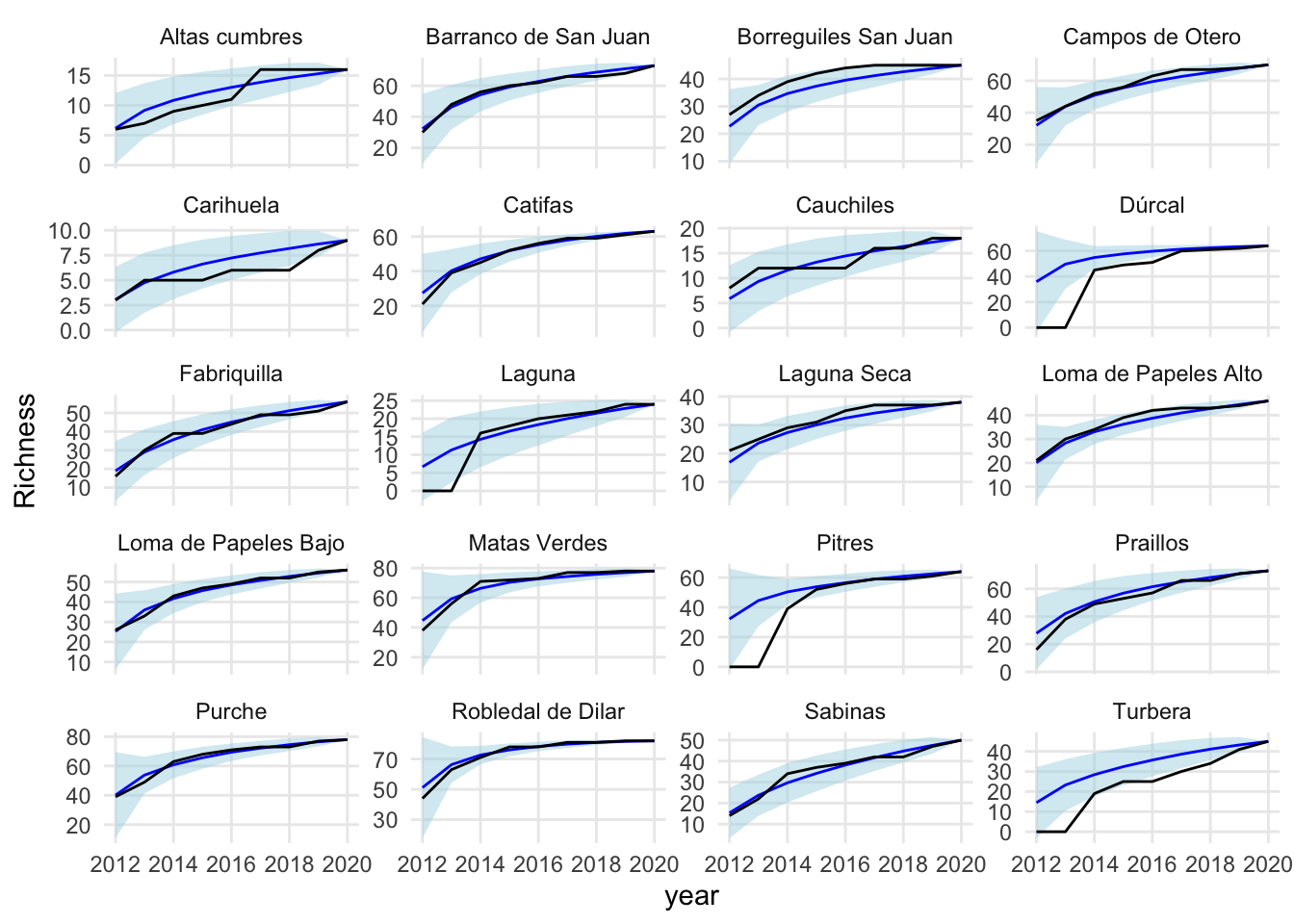
| Version | Author | Date |
|---|---|---|
| f07aef2 | ajpelu | 2022-07-11 |
dev.off()null device
1 Curvas Rarefaccion
mm <- m %>%
  inner_join(
    transectos %>% dplyr::select(transecto, site)) %>%
  relocate(y2018, .after=y2017) %>%
  ungroup() %>% rowwise() %>%
  mutate(abun = sum(across(starts_with("y")))) %>%
  dplyr::select(site, spabrev, abun) %>%
  pivot_wider(names_from = site, values_from = abun, values_fill = 0) %>%
  column_to_rownames("spabrev") %>% as.data.frame()

f <- iNEXT(mm, datatype = "abundance")
df <-  fortify(f, type = 1)


df.point <- df[which(df$method=="observed"),]
df.line <- df[which(df$method!="observed"),]
df.line$method <- factor(df.line$method,
 c("interpolated", "extrapolated"),
 c("interpolation", "extrapolation"))

plot_rarefy <- df %>%
  ggplot(aes(x=x, y=y)) +
  geom_point(size=2, data=df.point) +
  geom_line(aes(linetype=method), data=df.line) +
 geom_ribbon(aes(ymin=y.lwr, ymax=y.upr,
                 colour=NULL), alpha=0.2) +
  facet_wrap(~site, nrow = 5, scales = "free") +
  theme_minimal() +
  xlab("Number of individuals") +
  ylab("Species Diversity") +
  theme(legend.position = "bottom",
        legend.title=element_blank(),
        text=element_text(size=12))
plot_rarefy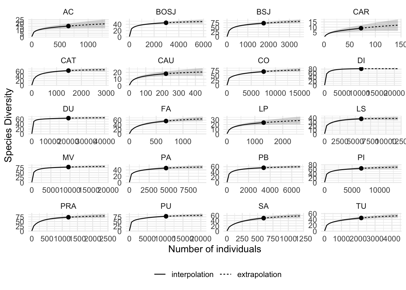
| Version | Author | Date |
|---|---|---|
| 9471064 | ajpelu | 2022-07-12 |
ggsave(here::here("figs/plot_rarefaction.pdf"),
       device = "pdf",
       width = 12, height = 11)
plot_rarefy 
| Version | Author | Date |
|---|---|---|
| 9471064 | ajpelu | 2022-07-12 |
dev.off()null device
1
sessionInfo()R version 4.0.2 (2020-06-22)
Platform: x86_64-apple-darwin17.0 (64-bit)
Running under: macOS Catalina 10.15.7
Matrix products: default
BLAS: /Library/Frameworks/R.framework/Versions/4.0/Resources/lib/libRblas.dylib
LAPACK: /Library/Frameworks/R.framework/Versions/4.0/Resources/lib/libRlapack.dylib
locale:
[1] en_US.UTF-8/en_US.UTF-8/en_US.UTF-8/C/en_US.UTF-8/en_US.UTF-8
attached base packages:
[1] stats graphics grDevices utils datasets methods base
other attached packages:
[1] iNEXT_2.0.20 writexl_1.3.1 vegan_2.5-7 lattice_0.20-41
[5] permute_0.9-5 DT_0.17 lubridate_1.7.10 here_1.0.1
[9] janitor_2.1.0 readxl_1.3.1 forcats_0.5.1 stringr_1.4.0
[13] dplyr_1.0.6 purrr_0.3.4 readr_1.4.0 tidyr_1.1.3
[17] tibble_3.1.2 ggplot2_3.3.5 tidyverse_1.3.1 workflowr_1.7.0
loaded via a namespace (and not attached):
[1] nlme_3.1-152 fs_1.5.0 httr_1.4.2 rprojroot_2.0.2
[5] tools_4.0.2 backports_1.2.1 bslib_0.3.1 utf8_1.1.4
[9] R6_2.5.1 DBI_1.1.1 mgcv_1.8-33 colorspace_2.0-2
[13] withr_2.4.1 tidyselect_1.1.1 processx_3.5.1 compiler_4.0.2
[17] git2r_0.28.0 textshaping_0.3.2 cli_2.5.0 rvest_1.0.0
[21] xml2_1.3.2 labeling_0.4.2 sass_0.4.1 scales_1.1.1.9000
[25] callr_3.7.0 systemfonts_1.0.0 digest_0.6.27 rmarkdown_2.14
[29] pkgconfig_2.0.3 htmltools_0.5.2 highr_0.8 dbplyr_2.1.1
[33] fastmap_1.1.0 htmlwidgets_1.5.4 rlang_0.4.12 rstudioapi_0.13
[37] farver_2.1.0 jquerylib_0.1.3 generics_0.1.0 jsonlite_1.7.2
[41] crosstalk_1.1.1 magrittr_2.0.1 Matrix_1.3-2 Rcpp_1.0.7
[45] munsell_0.5.0 fansi_0.4.2 lifecycle_1.0.1 stringi_1.7.4
[49] whisker_0.4 yaml_2.2.1 snakecase_0.11.0 MASS_7.3-53
[53] plyr_1.8.6 grid_4.0.2 parallel_4.0.2 promises_1.2.0.1
[57] crayon_1.4.1 haven_2.3.1 splines_4.0.2 hms_1.0.0
[61] knitr_1.31 ps_1.5.0 pillar_1.6.1 reshape2_1.4.4
[65] reprex_2.0.0 glue_1.4.2 evaluate_0.14 getPass_0.2-2
[69] modelr_0.1.8 vctrs_0.3.8 httpuv_1.5.5 cellranger_1.1.0
[73] gtable_0.3.0 assertthat_0.2.1 xfun_0.30 broom_0.7.9
[77] later_1.1.0.1 ragg_1.1.1 cluster_2.1.0 ellipsis_0.3.2