analysis peak
Antonio J.
Pérez-Luque

Last updated: 2023-07-26
Checks: 7 0
Knit directory: ms_mariposas_pheno/
This reproducible R Markdown analysis was created with workflowr (version 1.7.0). The Checks tab describes the reproducibility checks that were applied when the results were created. The Past versions tab lists the development history.
Great! Since the R Markdown file has been committed to the Git repository, you know the exact version of the code that produced these results.
Great job! The global environment was empty. Objects defined in the global environment can affect the analysis in your R Markdown file in unknown ways. For reproduciblity it’s best to always run the code in an empty environment.
The command set.seed(20230601) was run prior to running
the code in the R Markdown file. Setting a seed ensures that any results
that rely on randomness, e.g. subsampling or permutations, are
reproducible.
Great job! Recording the operating system, R version, and package versions is critical for reproducibility.
Nice! There were no cached chunks for this analysis, so you can be confident that you successfully produced the results during this run.
Great job! Using relative paths to the files within your workflowr project makes it easier to run your code on other machines.
Great! You are using Git for version control. Tracking code development and connecting the code version to the results is critical for reproducibility.
The results in this page were generated with repository version af43feb. See the Past versions tab to see a history of the changes made to the R Markdown and HTML files.
Note that you need to be careful to ensure that all relevant files for
the analysis have been committed to Git prior to generating the results
(you can use wflow_publish or
wflow_git_commit). workflowr only checks the R Markdown
file, but you know if there are other scripts or data files that it
depends on. Below is the status of the Git repository when the results
were generated:
Ignored files:
    Ignored:    .Rhistory
    Ignored:    .Rproj.user/
    Ignored:    data/raw_data/.DS_Store

Untracked files:
    Untracked:  data/best_models_prec.csv
    Untracked:  data/best_models_prec.xlsx
    Untracked:  data/best_models_temp.csv
    Untracked:  data/best_models_temp.xlsx
    Untracked:  data/doy_medio_sp.csv
    Untracked:  data/doy_medio_sp.xlsx
    Untracked:  data/models_prec_scaled.csv
    Untracked:  data/models_prec_scaled.xlsx
    Untracked:  data/models_tmed_scaled.csv
    Untracked:  data/models_tmed_scaled.xlsx

Unstaged changes:
    Modified:   analysis/climate_sensibility.Rmd
    Modified:   analysis/index.Rmd
    Modified:   data/models_prec.csv
    Modified:   data/models_prec.xlsx
    Modified:   data/models_tmed.csv
    Modified:   data/models_tmed.xlsx
    Modified:   data/selected_species.csv
Note that any generated files, e.g. HTML, png, CSS, etc., are not included in this status report because it is ok for generated content to have uncommitted changes.
These are the previous versions of the repository in which changes were
made to the R Markdown (analysis/analysis_peak.Rmd) and
HTML (docs/analysis_peak.html) files. If you’ve configured
a remote Git repository (see ?wflow_git_remote), click on
the hyperlinks in the table below to view the files as they were in that
past version.
| File | Version | Author | Date | Message |
|---|---|---|---|---|
| Rmd | af43feb | ajpelu | 2023-07-26 | add peak analysis |
| Rmd | fad23da | ajpelu | 2023-07-26 | update |
| html | fad23da | ajpelu | 2023-07-26 | update |
| html | 51eb91c | ajpelu | 2023-06-05 | Build site. |
| Rmd | 41ef77d | ajpelu | 2023-06-05 | add mean doy vs trend |
| html | c483988 | ajpelu | 2023-06-05 | Build site. |
| Rmd | 2b31d24 | ajpelu | 2023-06-05 | add selected species |
| html | 0e4287f | ajpelu | 2023-06-02 | Build site. |
| Rmd | 7ca3dcc | ajpelu | 2023-06-02 | update |
| Rmd | 1175615 | ajpelu | 2023-06-02 | update peak |
| Rmd | 1418e7a | ajpelu | 2023-06-01 | update computation of trends |
| Rmd | e3a3af1 | ajpelu | 2023-06-01 | add peak analysis |
| Rmd | d06a05b | ajpelu | 2023-06-01 | update |
Introduction
library(tidyverse)
library(here)
library(janitor)
library(lubridate)
library(ggpubr)
library(Kendall)
library(trend)
library(DT)
library(vroom)
df_doy <- vroom::vroom(here::here("data/doy_peak_sps.csv"))
transectos <- vroom::vroom(here::here("data/transectos_metadata.csv"))Exploratory analysis
First, we examine how the day of the year (doy) at which the maximum peak occurs varies throughout the years for each species and site. We create a custom function to generate a plot for each species faceted by site. All the pdfs generated are stored here.
plot_trend_doy_all <- function(df, sp){
  p <- df |>
    filter(species == sp) |>
    mutate(abb = fct_reorder(abb_elev, altitud)) |>
    ggplot(aes(x=year, y=doy)) +
    geom_point() +
    facet_wrap(~abb) +
    geom_smooth(method = "lm", se = FALSE) +
    ggpubr::stat_cor(
      cor.coef.name = "R"
      # aes(label = after_stat(r.label))
      ) +
    theme_bw() +
    theme(
    panel.grid= element_blank(),
    strip.background = element_blank()) +
    ylab("Day of year") + xlab("Year") +
  labs(
    title = sp
  )  +
    scale_x_continuous(breaks = seq(min(df$year), max(df$year), by = 2))

  return(p)
  }
For instance, the following figure shows the data plot for Aglais urticae
# Get species
species <- unique(df_doy$species)

plot_trend_doy_all(df_doy, species[1])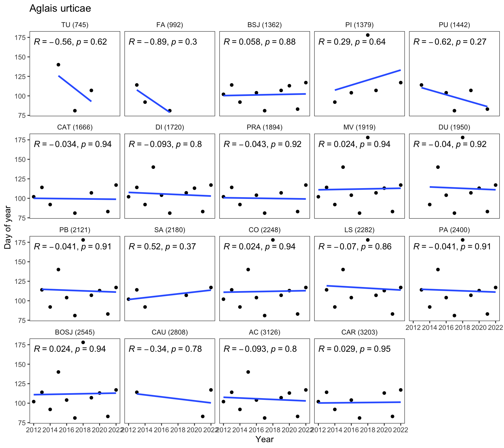
| Version | Author | Date |
|---|---|---|
| 0e4287f | ajpelu | 2023-06-02 |
# Generate PDF files for each species using purrr::map()
map(species, ~{
  sp <- .
  p <- plot_trend_doy_all(df_doy, sp)
  pdf_file <- here::here("output/pheno_peak_doy/", paste0(sp, ".pdf"))
  ggsave(filename = pdf_file, plot = p, device = "pdf")
})
How many data?
We would like to determine the number of sites where each species is
present (nsites), and also compute the number of sites
where the species has been recorded for at least 5 years
(nsites_higher4points)
npoints_sp_site <- df_doy |>
    ungroup() |>
    group_by(species, site_id, abb_elev) |>
  summarise(num_points = n())

nsites_by_sps <- npoints_sp_site |>
  group_by(species) |>
  summarise(nsites = n())

nsites_by_sps_4points <- npoints_sp_site |>
  filter(num_points > 4) |>
  group_by(species) |>
  summarise(nsites_higher4points = n())


ns <- nsites_by_sps |>
  full_join(nsites_by_sps_4points)

write_csv(ns, here::here("data/trends_peak_nsites.csv"))
Compute trends
We analyze the temporal trend of the date at which the peak flight occurs (DOY). We calculate the trends using both the Mann-Kendall and Sen’s slope methods, as well as linear methods, to assess how the DOY varies over time. We specifically focus on species where we have at least 5 data points, indicating that the species has been observed for a minimum of 5 years.
compute_trend <- function(y, x) {
  # Compute Mann-Kendall test
  mk <- MannKendall(y)
  mk_tau <- mk$tau
  mk_pvalue <- mk$sl

  # Compute Sen's slope
  sen <- trend::sens.slope(y)
  sen_slope <- unname(sen$estimates)
  sen_stats <- unname(sen$statistic)
  sen_pvalue <- unname(sen$p.value)

  # Compute LM
  model <- lm(y ~ x)
  lm_slope <- model$coefficients[2]
  lm_pvalue <- summary(model)$coefficients[2,4]
  lm_rsquared <- summary(model)$r.squared


  # Check for NULL values
  if (is.null(mk_tau)) mk_tau <- NA
  if (is.null(mk_pvalue)) mk_pvalue <- NA
  if (is.null(sen_slope)) sen_slope <- NA
  if (is.null(sen_stats)) sen_stats <- NA
  if (is.null(sen_pvalue)) sen_pvalue <- NA
  if (is.null(lm_slope)) lm_slope <- NA
  if (is.null(lm_pvalue)) lm_pvalue <- NA
  if (is.null(lm_rsquared)) lm_rsquared <- NA


  # Return results
  result <- data.frame(mk_tau = mk_tau,
                       mk_pvalue = mk_pvalue,
                       sen_slope = sen_slope,
                       sen_stats = sen_stats,
                       sen_pvalue = sen_pvalue,
                       lm_slope = lm_slope,
                       lm_pvalue = lm_pvalue,
                       lm_rsquared = lm_rsquared)

  return(result)
}
df_trends <- df_doy |>
ungroup() |>
group_by(species, site_id) |>
mutate(num_points = n()) |>
filter(num_points > 4) |>
group_modify(~compute_trend(.x$doy, .x$year)) |>
inner_join(transectos)
write_csv(df_trends, here::here("data/trends_peak.csv"))Apply only to selected species
Criteria for selected species: - Only univoltine species. - Non-migratory. - Exclude Favonius quercus - They must present data from at least five years (which do not have to be consecutive) - They don’t have to appear in more than one location to calculate their phenology
selected_sp <- vroom::vroom(here::here("data/selected_species.csv"),delim = ",")

df_trends_selected <- df_trends |>
  filter(species %in% selected_sp$sp)
We selected 45 species.
Explore the trends
By elevation
ggscatter(df_trends_selected,
          x = "altitud", y = "sen_slope",
          add = "reg.line",
          add.params = list(color = "blue", fill = "lightgray"),
          conf.int = TRUE,
          xlab = "Elevation (m)",
          ylab = "Sen's Slope") +
   stat_cor(method = "pearson", label.y = -10, label.x = 2500)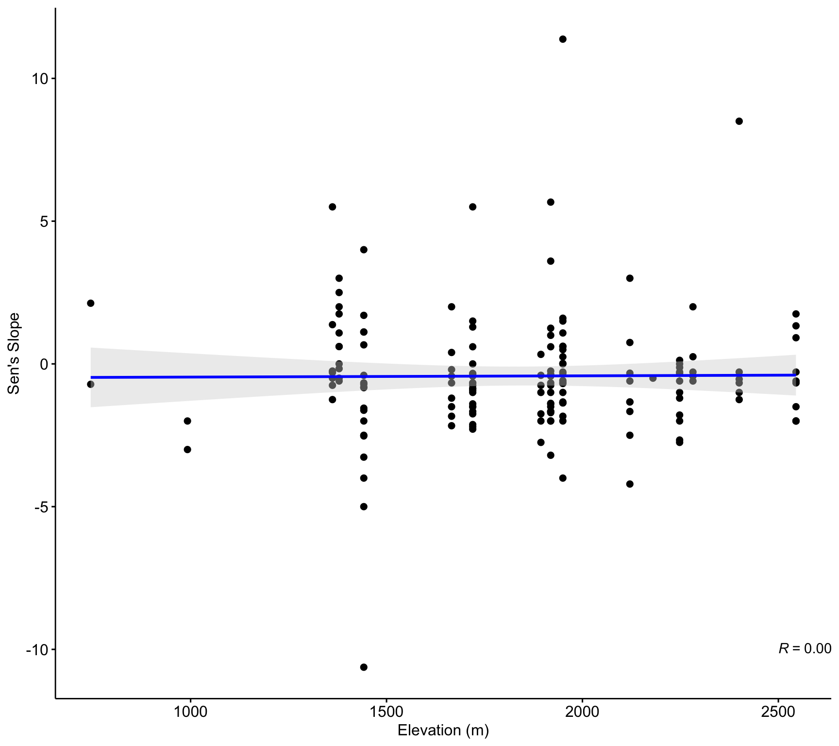
ggscatter(df_trends_selected,
          x = "altitud", y = "mk_tau",
          add = "reg.line",
          add.params = list(color = "blue", fill = "lightgray"),
          conf.int = TRUE,
          xlab = "Elevation (m)",
          ylab = "Mann-Kendall tau") +
   stat_cor(method = "pearson")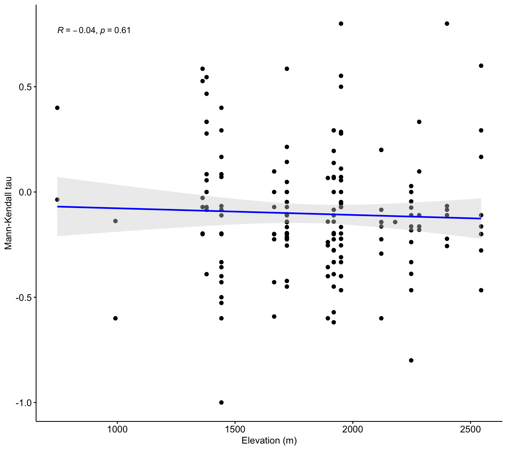
Explore by timing of the maximum
- First we computed the doy mean for each specie
doy_mean <- df_doy |>
  group_by(species) |>
  summarise(mean = mean(doy, na.rm = TRUE),
            median = median(doy, na.rm = TRUE),
            sd = sd(doy, na.rm = TRUE),
            se = sd(doy, na.rm = TRUE) / sqrt(n()),
            n = length(doy))

# df_doy |>
#   group_by(species, site_id) |>
#   summarise(mean = mean(doy, na.rm = TRUE),
#             median = median(doy, na.rm = TRUE),
#             sd = sd(doy, na.rm = TRUE),
#             se = sd(doy, na.rm = TRUE) / sqrt(n()),
#             n = length(doy))
doy_mean |>
ggplot(aes(x=forcats::fct_reorder(species, mean), y = mean)) + geom_point() +
geom_errorbar(aes(ymin = mean - se, ymax= mean + se)) +
coord_flip() +
theme_bw() +
theme(
panel.grid.major.x = element_blank(),
panel.grid.minor.x = element_blank()
) +
xlab("") + ylab("DOY")df_doy |>
ggplot(aes(x=reorder(species, doy, mean), y = doy)) + geom_point(size=.5, colour = "gray") +
stat_summary(fun.data = mean_sd, geom = "pointrange") +
coord_flip() +
theme_bw() +
theme(
panel.grid.major.x = element_blank(),
panel.grid.minor.x = element_blank()
) +
xlab("") + ylab("DOY") +
scale_y_continuous(breaks = seq(0, max(df_doy$doy), by = 20)) 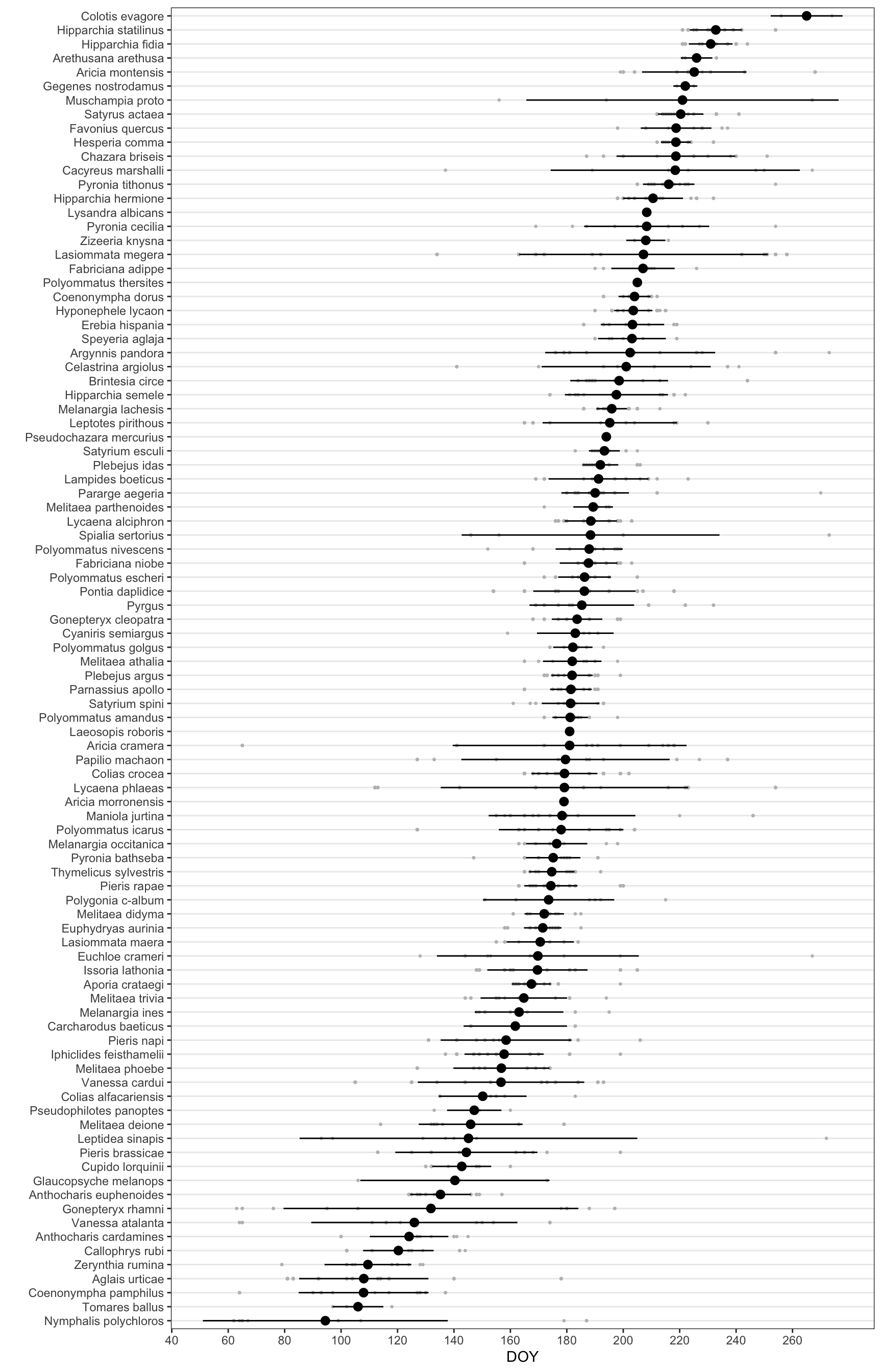
| Version | Author | Date |
|---|---|---|
| c483988 | ajpelu | 2023-06-05 |
Only for selected species
df_doy |>
  filter(species %in% selected_sp$sp) |>
  ggplot(aes(x=reorder(species, doy, mean), y = doy)) + geom_point(size=.5, colour = "gray") +
  stat_summary(fun.data = mean_sd, geom = "pointrange") +
  coord_flip() +
  theme_bw() +
  theme(
    panel.grid.major.x = element_blank(),
    panel.grid.minor.x = element_blank()
  ) +
  xlab("") + ylab("DOY") +
scale_y_continuous(breaks = seq(0, max(df_doy$doy), by = 20)) 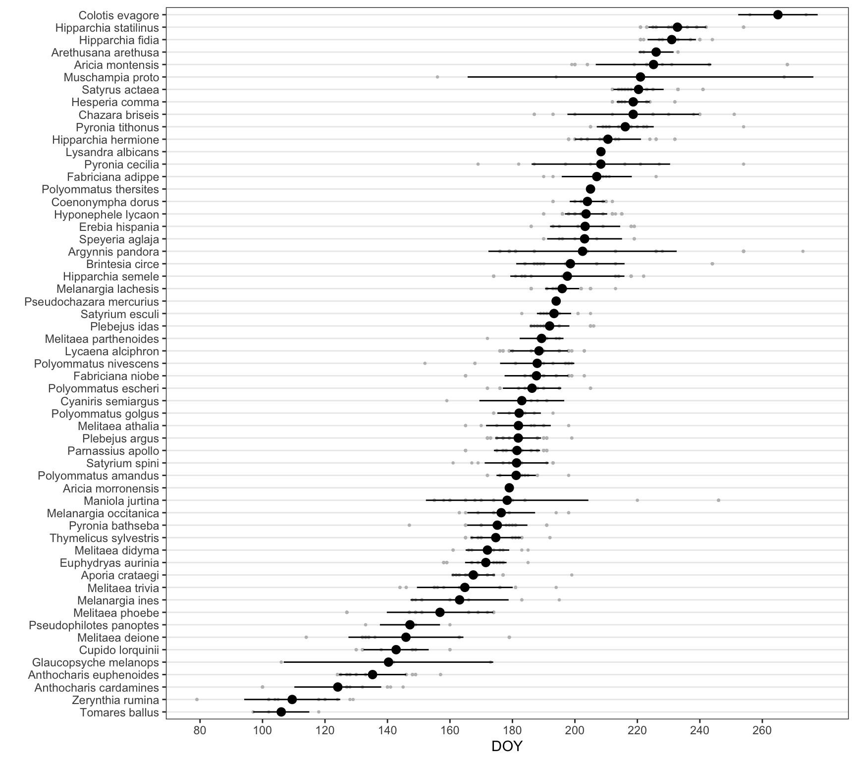
Explore by doy_mean
df_trends_selected_mean <- df_trends_selected |>
  group_by(species) |>
  summarise(tau_mean = mean(mk_tau),
            tau_sd = sd(mk_tau, na.rm = TRUE),
            ta_se = sd(mk_tau, na.rm = TRUE) / sqrt(n()),
            sen_mean = mean(sen_slope),
            sen_sd = sd(sen_slope, na.rm = TRUE),
            sen_se = sd(sen_slope, na.rm = TRUE) / sqrt(n())
            )

d <- inner_join(
  df_trends_selected_mean,
  (doy_mean |>
  rename(doy_mean = mean,
         doy_se = se,
         doy_sd = sd))
)
d |>
ggplot(aes(doy_mean, y = sen_mean)) +
geom_point() +
theme_bw() +
geom_smooth() +
xlab("DOY") +
ylab("Sen's slope")d |>
ggplot(aes(doy_mean, y = mk_tau)) +
geom_point() +
theme_bw() +
geom_smooth() +
xlab("DOY") +
ylab("Sen's slope")ggscatter(d,
x = "doy_mean", y = "tau_mean",
conf.int = TRUE,
xlab = "DOY",
ylab = "Mann-Kendall tau") +
geom_smooth(method = "loess", formula = y ~ x) +
geom_smooth(method = "lm", se = FALSE, colour = "black") 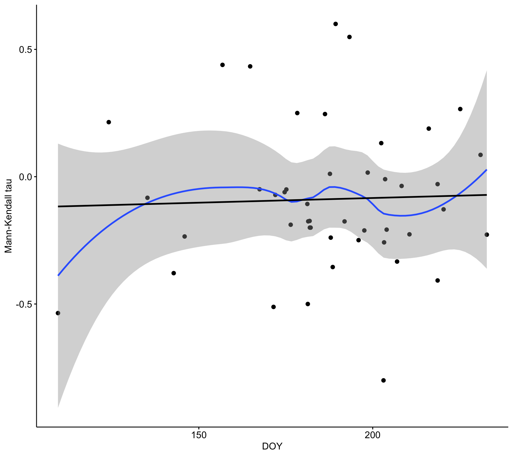
ggscatter(d,
          x = "doy_mean", y = "sen_mean",
          conf.int = TRUE,
          xlab = "DOY",
          ylab = "Sen's Slope") +
     geom_smooth(method = "loess", formula = y ~ x) +
geom_smooth(method = "lm", se = FALSE, colour = "black") 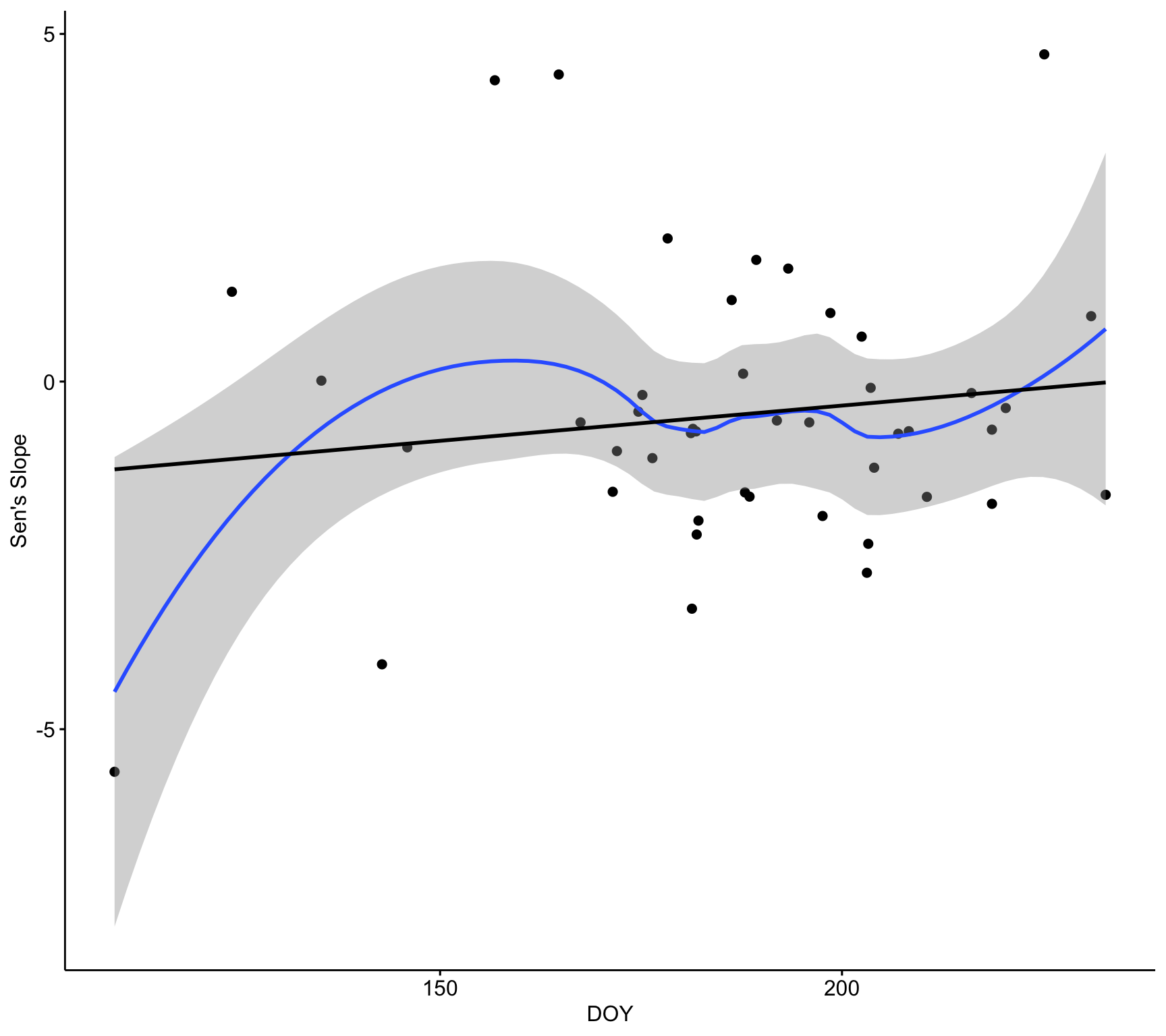
sessionInfo()R version 4.2.3 (2023-03-15)
Platform: x86_64-apple-darwin17.0 (64-bit)
Running under: macOS Big Sur ... 10.16
Matrix products: default
BLAS: /Library/Frameworks/R.framework/Versions/4.2/Resources/lib/libRblas.0.dylib
LAPACK: /Library/Frameworks/R.framework/Versions/4.2/Resources/lib/libRlapack.dylib
locale:
[1] en_US.UTF-8/en_US.UTF-8/en_US.UTF-8/C/en_US.UTF-8/en_US.UTF-8
attached base packages:
[1] stats graphics grDevices utils datasets methods base
other attached packages:
[1] vroom_1.6.3 DT_0.26 trend_1.1.4 Kendall_2.2.1
[5] ggpubr_0.4.0 janitor_2.1.0 here_1.0.1 lubridate_1.9.2
[9] forcats_1.0.0 stringr_1.5.0 dplyr_1.1.0 purrr_1.0.1
[13] readr_2.1.4 tidyr_1.3.0 tibble_3.1.8 ggplot2_3.4.1
[17] tidyverse_2.0.0 workflowr_1.7.0
loaded via a namespace (and not attached):
[1] httr_1.4.4 sass_0.4.5 splines_4.2.3 bit64_4.0.5
[5] jsonlite_1.8.4 carData_3.0-5 bslib_0.4.2 getPass_0.2-2
[9] highr_0.10 yaml_2.3.7 lattice_0.20-45 pillar_1.8.1
[13] backports_1.4.1 glue_1.6.2 digest_0.6.31 promises_1.2.0.1
[17] ggsignif_0.6.3 snakecase_0.11.0 colorspace_2.0-3 Matrix_1.5-3
[21] htmltools_0.5.4 httpuv_1.6.8 pkgconfig_2.0.3 broom_1.0.4
[25] scales_1.2.1 processx_3.7.0 whisker_0.4 later_1.3.0
[29] tzdb_0.3.0 timechange_0.1.1 git2r_0.30.1 mgcv_1.8-42
[33] farver_2.1.1 generics_0.1.3 car_3.1-0 ellipsis_0.3.2
[37] cachem_1.0.6 withr_2.5.0 cli_3.6.0 magrittr_2.0.3
[41] crayon_1.5.2 evaluate_0.19 ps_1.7.1 fs_1.6.2
[45] fansi_1.0.3 nlme_3.1-162 rstatix_0.7.0 tools_4.2.3
[49] hms_1.1.2 lifecycle_1.0.3 extraDistr_1.9.1 munsell_0.5.0
[53] callr_3.7.3 compiler_4.2.3 jquerylib_0.1.4 rlang_1.1.0
[57] grid_4.2.3 rstudioapi_0.14 htmlwidgets_1.6.2 crosstalk_1.2.0
[61] labeling_0.4.2 rmarkdown_2.19 boot_1.3-28.1 gtable_0.3.1
[65] abind_1.4-5 R6_2.5.1 knitr_1.41 fastmap_1.1.0
[69] bit_4.0.4 utf8_1.2.2 rprojroot_2.0.3 stringi_1.7.8
[73] parallel_4.2.3 Rcpp_1.0.10 vctrs_0.6.0 tidyselect_1.2.0
[77] xfun_0.39