The problem
Welfare, development or living standards are multidimensional
concepts. No single variable (income, GDP, etc.) fully captures them,
but combining many indicators into one synthetic measure raises a hard
question: how do you aggregate variables expressed in different units
and, above all, avoid double-counting the information that several
correlated indicators share? The P_2
distance (Pena, 1977) was designed to
solve exactly this problem. It is a distance-based synthetic indicator:
instead of choosing arbitrary weights for each variable, it measures how
far each unit of analysis (a region, a municipality, a household…) lies
from a reference situation, and it corrects that measure so
that indicators carrying redundant (correlated) information are not
counted twice. Bonet-García et al. (2015)
used the p2distance package to build such an indicator of
human well-being for Andalusian municipalities, which is a good worked
illustration of the method described below.
How the P2 distance is computed
The p2distance() function implements the algorithm
described in Bonet-García et al. (2015)
(following Pena (1977), and Montero et al. (2010)). The explanation below
follows the notation of that paper.
1. The data matrix and the reference vector
The starting point is a matrix X of order (m, n), where m is the number of spatial (or statistical) units (e.g. municipalities, countries, households) and n is the number of variables (indicators). Each element x_{ri} is the value of variable i in unit r.
To measure how far each unit is from an ideal or reference situation,
a reference vector X_* =
(x_{*1}, x_{*2}, \ldots, x_{*n}) must be defined: one reference
value per variable. Any vector that represents the condition against
which units are to be compared can be used (the minimum, the maximum, an
average, a user-defined target, etc.). The minimum value is often used
in sociological studies (Rodríguez Martín, 2011;
Somarriba & Pena, 2009; Zarzosa & Somarriba, 2012), which
is the default used by makeReferenceVector(); but any other
vector that reflects the ideal condition against which the units are to
be compared can also be used.
2. Partial distances
For every variable, the distance between each unit and the reference value is calculated:
d_{ri} = |x_{ri} - x_{*i}|, \qquad r = 1, \ldots, m; \; i = 1, \ldots, n \qquad (\text{Eq. 1})
The absolute value is used so that positive and negative deviations from the reference are treated the same way (Somarriba et al., 2014).
Because variables are measured in different units, each partial distance is standardized by dividing it by the standard deviation of that variable, \sigma_i, giving d_{ri}/\sigma_i.
3. The Fréchet Distance
Summing the standardized partial distances across all variables gives the Fréchet Distance:
FD(r) = \sum_{i=1}^{n} \frac{d_{ri}}{\sigma_i} = \sum_{i=1}^{n} \frac{|x_{ri}-x_{*i}|}{\sigma_i}, \qquad r = 1, \ldots, m \qquad (\text{Eq. 2})
FD(r) is the maximum value the P_2 distance can reach for unit r. The FD concept of distance is valid only in a theoretical situation of uncorrelated indicators. However, it is common to find direct relationships between the partial indicators, which implies that FD includes duplicate information.
4. The correction factor
To remove that redundancy, each partial indicator is weighted by a correction factor (1 - R^2_{i,i-1,\ldots,1}), where R^2_{i,i-1,\ldots,1} is the coefficient of determination of the linear regression of indicator i on all the indicators that have already entered the index (i-1, i-2, \ldots, 1). This coefficient measures the proportion of the variance of indicator i that is already explained by (linearly dependent on) the indicators already included. The factor (1 - R^2) therefore keeps only the genuinely new information that indicator i contributes and discards what is redundant with the indicators before it (Pena, 1977). If all the indicators are mutually uncorrelated, every R^2 = 0 and the P_2 distance simply equals FD.
5. The P2 distance
Applying the correction factor to every term of the sum gives the P_2 distance:
P_2(r) = \sum_{i=1}^{n} \left\{ \left(\frac{d_{ri}}{\sigma_i}\right)\left(1 - R^2_{i,i-1,i-2,\ldots,1}\right) \right\}, \qquad r = 1, \ldots, m \qquad (\text{Eq. 3})
6. Ordering the variables, and iterating to convergence
The equation for P_2 depends on the
order in which variables enter the index: the regression used
for the correction factor of variable i
is always on the variables that came before it. Deciding that order is
not arbitrary: p2distance() uses the iterative procedure of
Montero et al. (2010) to find it:
- Compute the partial indicators d_{ri}/\sigma_i from the data matrix and the reference vector (Eq. 1).
- Compute the Fréchet Distance FD(r) for every unit (Eq. 2).
- Determine the order of entrance of the variables: since FD already summarizes the information of all the partial indicators, the variable most strongly correlated with FD is the one that contributes most variance to the index, so it enters first. The correlation of every partial indicator with FD ranks the remaining variables for this first pass.
- Compute the correction factors (1-R^2) for each variable, following that order.
- Compute a first P_2 distance, P_2^{1}, applying Eq. 3 with the order and correction factors from steps 3–4.
- Check for convergence: the correlation of every variable with this new P_2^{1} index is used to re-rank the order of entrance, and the whole procedure (steps 3–5) is repeated to obtain P_2^{2}, then P_2^{3}, and so on. The algorithm stops as soon as two consecutive iterations agree — i.e. the first P_2^{j} for which P_2^{j} = P_2^{j+1} is the final P_2 distance returned for every unit.
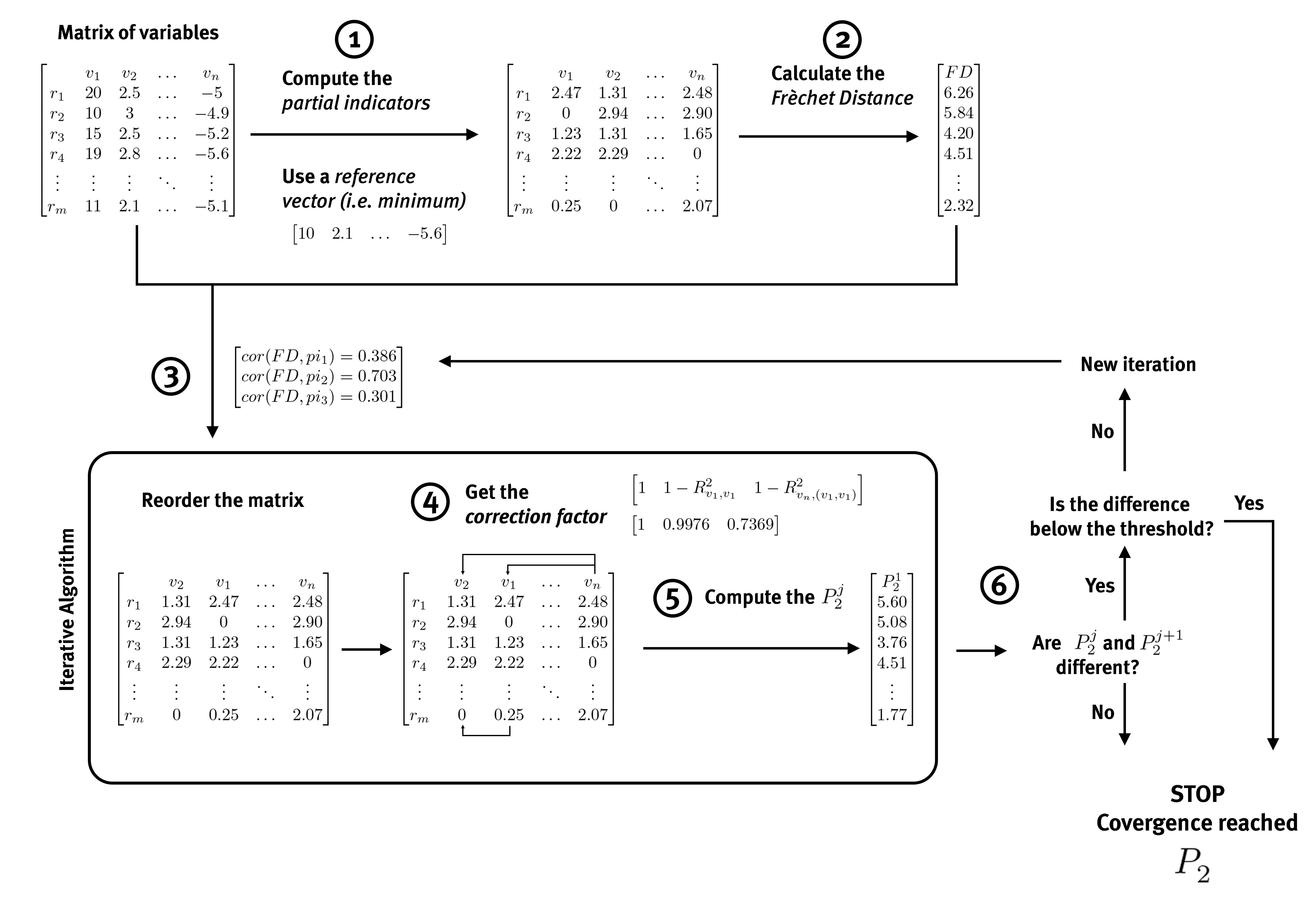
The following figure summarizes this procedure: (1) the partial indicators are computed from the initial data matrix using the reference vector; (2) the Fréchet Distance is computed; (3) the order of entrance of the variables is determined from the correlation between the partial indicators and FD; (4) once the matrix is reordered, the correction factor of each variable is obtained; (5) the first P_2 distance, P_2^{1}, is computed by applying Eq. (3); (6) the difference between P_2^{j} and P_2^{j-1} is evaluated (in the initial iteration, FD and P_2^{1} are compared) — if the difference is zero, the algorithm stops; otherwise, the matrix is reordered according to the correlation of the partial indicators with the last P_2^{j} obtained, and a new P_2 is computed.
A real-world application
Bonet-García et al. (2015) applied this method to compare human well-being in Andalusian municipalities (southern Spain) in 1989 and 2009, combining 22 socioeconomic indicators (population, health, employment, income, infrastructure, education, culture and social participation) into a single P_2 well-being index. Well-being increased significantly between the two years, and the increase was significantly larger in municipalities located within Natural or National Parks than in unprotected ones (well-being ratio 1.144 vs. 1.121, p = 0.0066), evidence, according to the authors, of a spatial association between long-term protected-area management and improvements in local human well-being. See the full paper for the complete indicator list, methodology and results.